Reinforcement Learning: Exploring the Latest Advancements and Innovations

Introduction to Reinforcement Learning

Reinforcement Learning (RL) is rapidly emerging as one of the most dynamic and innovative areas within artificial intelligence. This technology is not just a theoretical concept; it’s driving real-world changes and improvements across various sectors. Imagine machines that can learn from their experiences and make decisions in complex environments, just like humans do. That’s the essence of Reinforcement Learning (RL).

From robotics to game playing, RL is making waves by enabling systems to improve their performance through trial and error. For instance, RL algorithms are helping robots learn new tasks and adapt to their surroundings without human intervention. In the world of gaming, Reinforcement Learning (RL) is behind some of the most impressive feats, like beating human champions in complex games.

In this article, we will explore the basic principles of RL and explain how these principles are applied to real-world scenarios. We will also explore the latest advancements in the field, showcasing how RL is pushing the boundaries of what’s possible. Whether you’re just starting to explore AI or looking to deepen your understanding, this guide will provide valuable insights into the world of Reinforcement Learning (RL) and its growing impact on technology and society.

Understanding Reinforcement Learning (RL)

What is Reinforcement Learning?

Reinforcement Learning (RL) is a type of machine learning where an agent learns how to make decisions by interacting with an environment. Unlike other types of learning, such as supervised learning (where a model learns from a set of labeled examples), RL focuses on learning from the outcomes of its actions, guided by rewards or penalties.

In RL, the goal is for the agent to learn how to take actions that will lead to the highest total reward over time. It’s like teaching a robot how to navigate a maze by rewarding it when it makes progress and penalizing it when it hits dead ends.

Key Characteristics of RL:

• Trial and Error: The agent learns by trying different actions and seeing what happens. For example, if the agent is learning to play a game, it might try different moves to see which ones result in winning points. This process helps the agent understand which actions lead to better outcomes.
• Delayed Rewards: Sometimes, the results of an action are not immediate. For instance, if the agent makes a move that will only show its benefit later in the game, it has to learn that the move is valuable even though the reward isn’t instant. This makes learning a bit more complex, as the agent needs to connect its actions with rewards that come after some time.
• Exploration vs. Exploitation: The agent faces a key decision: should it explore new actions to see if they could be better, or should it exploit the actions that it already knows are effective? For example, if the agent knows that a certain move usually wins points, it might keep using that move (exploitation). However, it also needs to try new moves occasionally (exploration) to find even better strategies.

Simple Example:

Imagine training a dog to fetch a ball. The dog (agent) needs to learn that fetching the ball (action) and bringing it back (sequence of actions) will result in a treat (reward). The dog will try different strategies and eventually learn the optimal way to fetch the ball to maximize its treats.

Key Concepts in Reinforcement Learning

Agents and Environments

In Reinforcement Learning (RL), two main components are the agent and the environment.

• Agent: This is the learner or decision-maker. It could be a robot, a computer program, or any system that makes decisions. The agent’s job is to take actions based on its understanding of the environment to achieve its goals.
• Environment: This is everything the agent interacts with. It includes all the factors and conditions that affect the agent’s decisions. For example, if the agent is a robot navigating a maze, the maze itself is the environment. It reacts to the agent’s actions and provides feedback in the form of rewards or punishments.

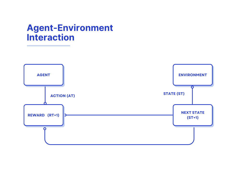
This diagram illustrates the interaction between an agent and an environment in the context of reinforcement learning. It shows the flow of actions and states as follows:

1. State (St): The current state of the environment as perceived by the agent.
2. Action (At): The action taken by the agent based on the current state.
3. Next State (St+1): The resulting state of the environment after the agent’s action.
4. Reward (Rt+1): The feedback received by the agent from the environment for the action taken.

The process is cyclic, with the agent continuously interacting with the environment, receiving new states and rewards, and updating its actions accordingly.

Rewards and Punishments

Rewards and punishments are essential for teaching an agent how to perform better. They provide feedback based on the agent’s actions, guiding it toward making better decisions in the future.

Rewards

• Rewards are positive feedbacks given to the agent when it takes actions that lead to good outcomes. For instance, if the agent successfully completes a task or moves closer to its goal, it receives a reward. The purpose of rewards is to encourage the agent to repeat actions that lead to positive outcomes. Over time, the agent learns to perform actions that maximize its total rewards.

Punishments

• Punishments are negative feedbacks given when the agent’s actions lead to poor outcomes. For example, if the agent makes a wrong move or fails to achieve its goal, it might receive a punishment. Punishments help the agent understand which actions to avoid.

Reward Function

The reward function is a critical component that defines how rewards and punishments are assigned. It maps each state-action pair to a reward, helping the agent understand the immediate benefit of an action.

Here’s how it works in practice:

def reward_function(state, action):
    if action == 'fetch' and state == 'ball_thrown':
        return 10  # positive reward for fetching the ball
    elif action == 'bark' and state == 'ball_thrown':
        return -1  # negative reward for barking instead of fetching
    else:
        return 0   # no reward for other actions

Example Explanation

• State: The current situation the agent is in. For instance, “ball_thrown” means the ball has been thrown.
• Action: What the agent decides to do. For example, “fetch” means the agent goes to fetch the ball, while “bark” means the agent barks.

In the above code:

• If the state is “ball_thrown” and the action is “fetch,” the agent receives a reward of 10. This positive reward encourages the agent to fetch the ball when it is thrown.
• The state is “ball_thrown” and the action is “bark,” the agent gets a punishment of -1. This negative reward discourages the agent from barking when it should fetch the ball.
• For any other state-action pair, the reward is 0, indicating no feedback for those actions.

By using rewards and punishments effectively, the agent learns to choose actions that lead to positive outcomes and avoid actions that result in negative outcomes. This learning process helps the agent improve its performance over time.

Policy and Value Functions

Policy

A policy is essentially the agent’s strategy or plan for choosing actions. It determines how the agent behaves at any given time, mapping states to actions. Think of it as a guide that tells the agent what to do in different situations.

• Simple Policy: This might involve always choosing the same action in a given state, regardless of the circumstances.
• Complex Policy: This can be more sophisticated, taking into account past experiences, current conditions, and potential future outcomes to decide the best action to take.

Value Functions

Value functions help the agent evaluate how beneficial it is to be in a certain state or to take a certain action. They are crucial for the agent to understand the long-term benefits of its actions.

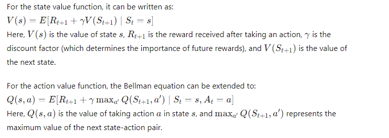
1. State Value Function (V(s)): This function measures how good it is for the agent to be in a particular state. It tells the agent the expected total reward it can get if it starts from that state and follows its policy from then on.
2. Action Value Function (Q(s, a)): Also known as the Q-function, this function measures how good a particular action is in a specific state. It tells the agent the expected reward of taking that action in that state and then following its policy in the future.

Bellman Equation

The Bellman equation is a fundamental formula in RL that helps compute the value of a state. It is a recursive equation that expresses the value of a state in terms of the rewards and the values of the next states.

Example Code

Here’s an example of how you might implement the Q-learning update rule, which uses the Bellman equation to update the Q-values:

import numpy as np

# Define the number of states and actions
num_states = 5  # Example number of states
num_actions = 3  # Example number of actions

# Initialize Q-table with zeros
Q = np.zeros((num_states, num_actions))

# Bellman update equation
def update_q(state, action, reward, next_state, alpha, gamma):
    best_next_action = np.argmax(Q[next_state])
    td_target = reward + gamma * Q[next_state, best_next_action]
    td_error = td_target - Q[state, action]
    Q[state, action] += alpha * td_error

# Example usage
alpha = 0.1  # learning rate
gamma = 0.9  # discount factor
state = 0
action = 1
reward = 10
next_state = 2

update_q(state, action, reward, next_state, alpha, gamma)

print("Updated Q-table:")
print(Q)

In this code:

• Q: The Q-table, which stores the Q-values for all state-action pairs.
• update_q: A function to update the Q-value for a given state-action pair using the Bellman equation.
• alpha: The learning rate, which determines how much new information overrides old information.
• gamma: The discount factor, which determines the importance of future rewards.
• state, action, reward, next_state: Example values showing how the Q-values are updated.

By updating the Q-values in this way, the agent learns to estimate the long-term value of its actions and can improve its policy to maximize rewards.

Output

Updated Q-table:

[[0. 1. 0.]
 [0. 0. 0.]
 [0. 0. 0.]
 [0. 0. 0.]
 [0. 0. 0.]]

Explanation

• Initial Q-table: The Q-table was initially filled with zeros.
• After update_q Call:
  • The Q-value for state = 0 and action = 1 was updated.
  • Given the example inputs, the value at Q[0, 1] has been updated to 1.0, reflecting the reward of 10 and the learning rate (alpha) of 0.1.

Next Steps

1. Further Testing: You might want to test the update_q function with different states, actions, rewards, and other parameters to ensure it works under various conditions.
2. Integration: Integrate this Q-learning update logic with a complete reinforcement learning environment where the agent interacts with the environment, collects rewards, and updates the Q-values accordingly.
3. Visualization: If you want to visualize how the Q-table evolves over time, you can add more sophisticated logging or plotting.

Recent Breakthroughs in Reinforcement Learning

Latest Advancements in Reinforcement Learning

Reinforcement Learning (RL) is rapidly evolving, thanks to new algorithms, increased computational power, and expanding applications. Here are some of the most notable recent advancements in the field:

Deep Reinforcement Learning Innovations

Combining Deep Learning with RL

Deep Reinforcement Learning (DRL) merges deep learning with Reinforcement Learning (RL) to solve complex tasks that involve high-dimensional data. Here’s how it works and why it’s powerful:

Deep Learning Models: DRL uses advanced neural networks to help RL handle complex problems. These neural networks can process and analyze large amounts of data, like images or sensor readings, and use this information to make decisions. This combination allows DRL to tackle tasks that were previously too difficult for traditional RL methods.

Key Advantages of DRL:

• Feature Extraction: Deep neural networks automatically find and extract important features from raw data. For example, in image data, these networks can identify objects, shapes, and patterns without needing manual feature engineering. This makes it easier for the RL agent to understand and act on complex inputs.
• Scalability: DRL can manage large-scale problems effectively. This is important for real-world applications, such as autonomous driving, where the system needs to process vast amounts of data and make quick decisions. DRL is also used in game playing, where agents can learn to play complex games like chess or Go by processing detailed game states.

Example: Training an Agent to Play Atari Games

A classic example of DRL is using a Deep Q-Network (DQN) to train an agent to play Atari games. Here’s a simplified explanation of how it works:

1. Game Screen (Pixels): The agent receives the game screen as input. This is a high-dimensional image made up of pixels.
2. Convolutional Neural Network (ConvNet): This network processes the game screen to extract useful features. It helps the agent understand important aspects of the image, like where objects are located or how the game environment looks.
3. Actions: The agent can choose from various actions, such as moving left, right, or firing in the game.
4. Q-Values: The ConvNet predicts the Q-values, which estimate the potential rewards of each action. The agent uses these predictions to decide the best action to take.

By combining deep learning with RL, DRL can solve problems that involve complex inputs and large action spaces, making it a powerful tool for many challenging applications.

Notable Algorithms: DQN, A3C, and PPO

DQN (Deep Q-Network)

Deep Q-Network (DQN) represents a significant advancement in Reinforcement Learning (RL) by combining Q-learning with deep neural networks. Here’s a breakdown of how DQN works and why it’s effective:

What is DQN?

• Q-Learning: This is a traditional RL method used to find the best action to take in each state by estimating Q-values (which predict future rewards).
• Deep Neural Networks: DQN uses neural networks to approximate these Q-values. This is especially useful when the state or action space is too large for traditional Q-learning to handle effectively.

How Does DQN Work?

1. Experience Replay: DQN stores past experiences in a memory buffer. Instead of learning from recent experiences only, it samples randomly from this buffer to train the network. This helps in breaking the correlation between consecutive experiences and makes training more stable.
2. Target Networks: DQN uses two networks:
   • Main Network: This is updated frequently based on recent experiences.
   • Target Network: This is a copy of the main network that is updated less frequently. It provides stable Q-value estimates for calculating the target values in the Q-learning update.

Example Code

Here’s how you can define a simple Q-network using TensorFlow and Keras:

import tensorflow as tf
from tensorflow.keras import layers

# Define the Q-network
def build_q_network(input_shape, num_actions):
    model = tf.keras.Sequential([
        layers.Conv2D(32, (8, 8), strides=4, activation='relu', input_shape=input_shape),
        layers.Conv2D(64, (4, 4), strides=2, activation='relu'),
        layers.Conv2D(64, (3, 3), strides=1, activation='relu'),
        layers.Flatten(),
        layers.Dense(512, activation='relu'),
        layers.Dense(num_actions)  # Output layer with num_actions nodes
    ])
    return model

# Example usage
input_shape = (84, 84, 4)  # Shape of the input data (e.g., game screen with 84x84 pixels and 4 frames)
num_actions = 4  # Number of possible actions (e.g., left, right, up, down)
q_network = build_q_network(input_shape, num_actions)

Explanation of the Code:

1. Input Shape: The input shape (84, 84, 4) represents the dimensions of the input data. In this case, it’s a screen with 84×84 pixels and 4 frames stacked together to capture motion.
2. Convolutional Layers: These layers help the network extract features from the input images. The Conv2D layers with different filter sizes and strides help in recognizing patterns and structures in the image.
3. Flatten Layer: This layer converts the 2D features into a 1D vector, which is then fed into the fully connected layers.
4. Dense Layers: These layers are fully connected and help the network learn complex representations. The final Dense layer outputs Q-values for each possible action.

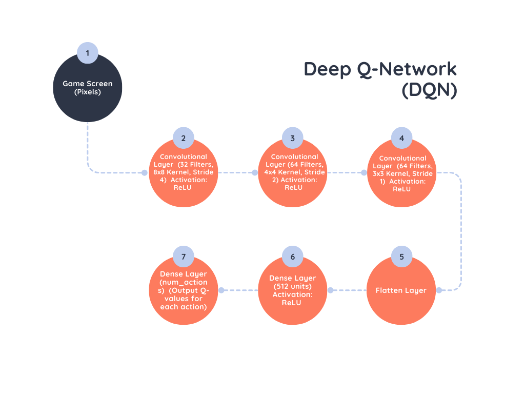
Here’s a diagram to illustrate this process:

Explanation:

1. Game Screen (Pixels): The input to the network, usually a sequence of frames from a game or environment.
2. Convolutional Layers: Three convolutional layers process the input images:
   • The first layer extracts features with 32 filters of size 8×8.
   • The second layer extracts more complex features with 64 filters of size 4×4.
   • The third layer further refines these features with 64 filters of size 3×3.
3. Flatten Layer: Converts the 2D feature maps into a 1D vector to feed into fully connected layers.
4. Dense Layers:
   • The first dense layer with 512 units processes the flattened features.
   • The final dense layer outputs the Q-values for each possible action, allowing the agent to decide which action to take based on the predicted rewards.

This architecture allows the DQN to handle complex, high-dimensional input data and make informed decisions based on learned features.

Must Read

• AI Pulse Weekly: December 2024 – Latest AI Trends and Innovations
• Can Google’s Quantum Chip Willow Crack Bitcoin’s Encryption? Here’s the Truth
• How to Handle Missing Values in Data Science
• Top Data Science Skills You Must Master in 2025
• How to Automating Data Cleaning with PyCaret

A3C (Asynchronous Advantage Actor-Critic)

A3C is an advanced reinforcement learning algorithm that enhances training by using multiple parallel environments. Here’s how it works and why it’s effective:

Key Features of A3C

1. Asynchronous Updates:
   • Multiple Agents: A3C runs several instances of the environment at the same time. Each instance trains a separate agent.
   • Global Model: These agents share and update a single global model. This means they learn from their own experiences and also from each other’s experiences.
   • Improved Exploration: With multiple agents exploring different parts of the environment simultaneously, A3C can discover more about the environment and learn better strategies.
   • Faster Training: Since the agents update the global model asynchronously, the training process is more efficient and converges faster to good solutions.
2. Advantage Function:
   • Actor-Critic Architecture: A3C uses two separate networks:
     • Actor Network: Decides what action to take based on the current state.
     • Critic Network: Evaluates how good the action taken by the actor is. It assesses the value of taking a specific action in a particular state.
   • Advantage Estimation: The advantage function measures how much better taking a particular action is compared to the average expected return. It helps in fine-tuning the actor’s decision-making process by providing a clearer understanding of which actions are more beneficial.

How It Works

1. Training with Multiple Environments: While each agent interacts with its own environment, it sends updates to a shared global model. This setup helps the agents learn faster and more effectively because they get a broader range of experiences.
2. Actor Network: The actor network proposes actions based on the state of the environment. For example, in a game, it might decide whether the agent should move left, right, or jump.
3. Critic Network: The critic network evaluates the action taken by the actor. It calculates how much reward the action is likely to produce compared to the average expected reward, providing feedback on whether the action was good or bad.
4. Updating the Model: The global model gets updated with contributions from all agents. This asynchronous updating ensures that the model improves steadily as more information is gathered from different agents.

By running multiple agents in parallel and using an actor-critic approach, A3C improves the learning efficiency and stability of reinforcement learning systems, making it a powerful tool for complex tasks.

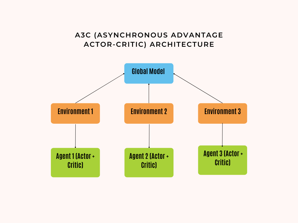
Here’s a diagram illustrating the A3C (Asynchronous Advantage Actor-Critic) architecture:

Explanation of the Diagram

1. Global Model:
   • This is the shared model that all agents update. It combines the knowledge from all the agents to improve learning efficiency and stability.
2. Environments:
   • Multiple instances of the environment run in parallel. Each environment interacts with a different agent, allowing for diverse experiences.
3. Agents:
   • Each agent interacts with its environment and consists of:
     • Actor Network: Decides which actions to take based on the state of the environment.
     • Critic Network: Evaluates the action taken by the actor by estimating how good it is compared to the average expected return.
4. Asynchronous Updates:
   • Agents send their updates to the global model independently. This means that the global model receives contributions from all agents asynchronously, which helps in faster and more effective learning.

In summary, the diagram shows how A3C uses multiple parallel agents and environments to update a global model, with each agent having its own actor and critic networks to decide and evaluate actions.

PPO (Proximal Policy Optimization)

Proximal Policy Optimization (PPO) is a reinforcement learning algorithm designed to provide a good balance between performance and stability. It improves the training of agents by making sure that updates to the policy are controlled, preventing drastic changes that can lead to instability.

Key Features of PPO

1. Clipped Objective:
   • Control Policy Changes: PPO uses a clipping mechanism in its objective function. This means it limits how much the policy can change during each update.
   • Prevent Instability: By clipping the objective function, PPO prevents the policy from making large updates that might destabilize the learning process.
2. Surrogate Objective:
   • Safe Updates: PPO uses a surrogate loss function to guide the policy updates. This function helps ensure that changes to the policy stay within a safe range, improving learning stability.
   • Optimization: The surrogate objective function helps in optimizing the policy efficiently while keeping updates within controlled limits.

Example Code

Here’s a basic example of defining a PPO policy network using TensorFlow:

import tensorflow as tf
from tensorflow.keras import layers

# Define the PPO policy network
class PPOPolicy(tf.keras.Model):
    def __init__(self, num_actions):
        super(PPOPolicy, self).__init__()
        self.dense1 = layers.Dense(128, activation='relu')
        self.dense2 = layers.Dense(128, activation='relu')
        self.policy_logits = layers.Dense(num_actions)  # Output layer for policy logits
        self.value = layers.Dense(1)  # Output layer for value function

    def call(self, inputs):
        x = self.dense1(inputs)
        x = self.dense2(x)
        return self.policy_logits(x), self.value(x)

# Example usage
num_actions = 4  # Number of possible actions
policy = PPOPolicy(num_actions)

Explanation of the Code

1. PPOPolicy Class:
   • __init__ Method: Initializes the PPO policy network with two hidden layers of 128 units each, using ReLU activation functions. It has:
     • Policy Logits: Outputs the action probabilities (or logits) for each action.
     • Value Function: Estimates the value of the current state.
   • call Method: Defines the forward pass through the network. It processes input data through the hidden layers and produces the policy logits and value function.

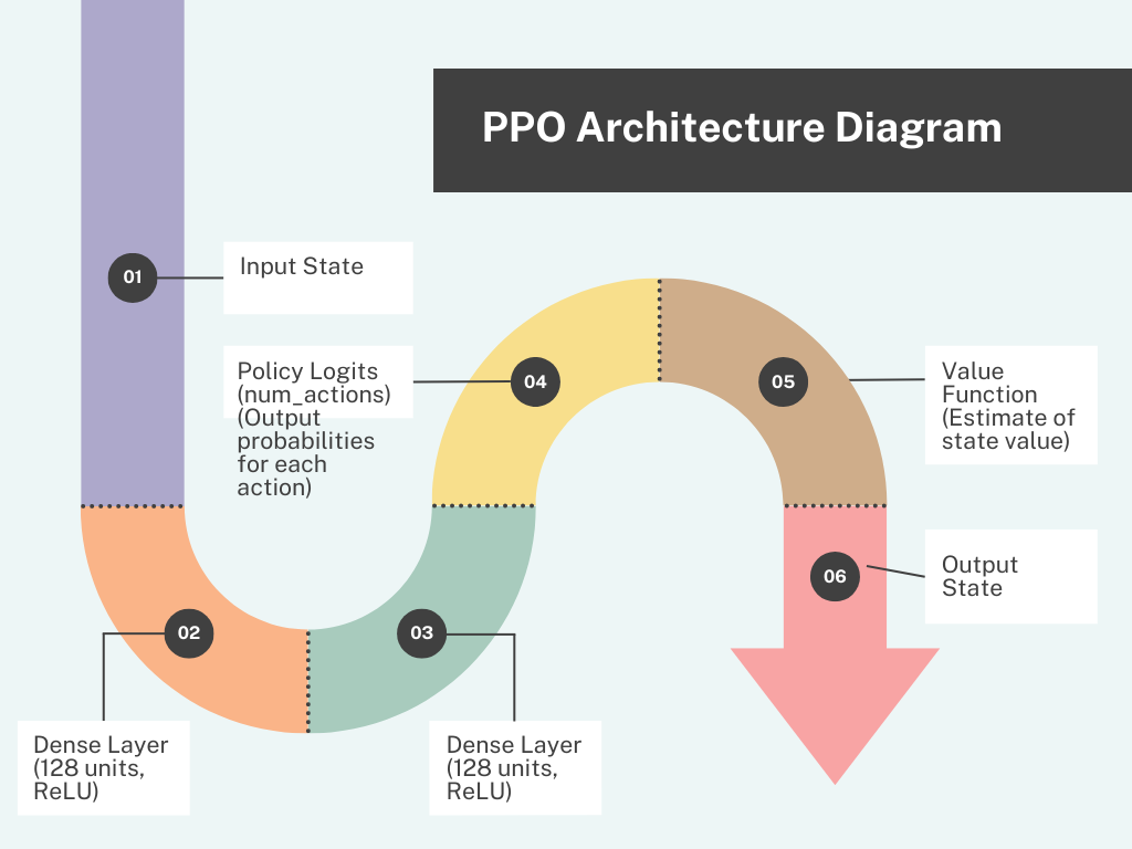
Diagram of PPO Architecture

Here’s a diagram to visualize how PPO works:

Explanation of the Diagram

1. Input State: The initial state input from the environment.
2. Dense Layers:
   • First Dense Layer: Processes the input state with 128 units and ReLU activation.
   • Second Dense Layer: Further processes the output with another 128 units and ReLU activation.
3. Policy Logits: Outputs the action probabilities for each possible action, helping the agent decide which action to take.
4. Value Function: Estimates the value of the current state, which helps the agent understand how favorable the state is.
5. Output State: Represents the result after taking an action based on the policy logits and evaluating the state with the value function. This is the new state that the agent will encounter after performing the action.

PPO effectively controls policy updates through its clipped objective and surrogate loss, making it a strong method for training reinforcement learning agents.

Reinforcement Learning in Robotics

Reinforcement Learning (RL) is transforming robotics by enhancing how robots learn to perform tasks and navigate complex environments. Let’s break down two key applications: autonomous navigation systems and robot learning from demonstrations.

Autonomous Navigation Systems

Autonomous navigation involves enabling robots to move and operate independently within their environment. Here’s a closer look at how this is achieved:

1. Sim-to-Real Transfer:
   • Training in Simulation: Initially, robots are trained in simulated environments. These simulations create virtual scenarios that mimic real-world conditions but are faster and cheaper to test. This step allows robots to practice and learn without physical risks.
   • Real-World Application: Once the robot performs well in simulations, the learned behaviors are transferred to real-world robots. This approach minimizes the time and resources needed for physical training and allows for quick adjustments based on simulation results.
2. Sensor Integration:
   • Perception: To navigate effectively, robots need to understand their surroundings. They use various sensors to gather information:
     • LIDAR: Measures distances to objects by bouncing laser beams off surfaces. It helps create a detailed map of the environment.
     • Cameras: Capture visual information that helps in recognizing objects, detecting obstacles, and understanding the scene.
   • Integration: By combining data from different sensors, robots can build a comprehensive understanding of their environment, which is crucial for safe and efficient navigation.

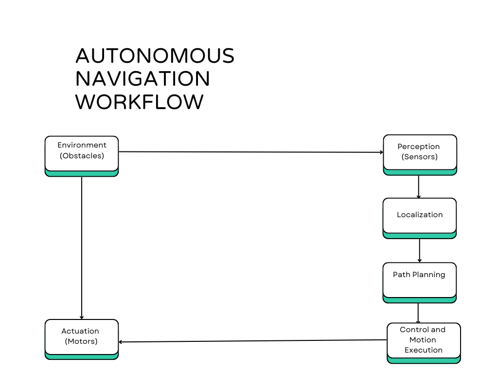
Here’s a diagram to visualize Autonomous Navigation Workflow:

Explanation:

1. Environment: Represents the robot’s surroundings, including obstacles and other elements.
2. Perception: Sensors (like LIDAR and cameras) gather data about the environment.
3. Localization: Determines the robot’s position within the environment using sensor data.
4. Path Planning: Plans a route for the robot to follow from its current position to its goal, avoiding obstacles.
5. Control and Motion Execution: Uses actuators (motors) to move the robot according to the planned path.

Robot Learning from Demonstrations

Learning from Demonstrations (LfD) allows robots to learn new tasks by observing humans perform them. This approach simplifies the training process and enhances the robot’s ability to handle complex tasks.

1. Imitation Learning:
   • Mimicking Actions: In this approach, robots learn by imitating the actions demonstrated by humans. For example, if a human shows a robot how to assemble a part, the robot tries to replicate those movements to complete the task.
   • Training: The robot records demonstrations, learns from them, and develops a policy or set of rules based on observed actions.
2. Inverse Reinforcement Learning:
   • Inferring Rewards: Instead of being given explicit rewards, the robot deduces the reward function from the demonstrations. This means the robot learns what actions are considered good or bad based on the behavior observed during demonstrations.
   • Policy Learning: By understanding the underlying reward structure, the robot can create a policy that mimics the demonstrated behavior and adapts it to new situations.

Example Code: Imitation Learning

import numpy as np

# Example of imitation learning using recorded demonstrations
def learn_from_demonstrations(demonstrations):
    policy = {}
    for state, action in demonstrations:
        policy[state] = action
    return policy

# Example usage
demonstrations = [
    (state1, action1),
    (state2, action2),
    # Additional state-action pairs
]
learned_policy = learn_from_demonstrations(demonstrations)

Explanation:

• Function learn_from_demonstrations: This function creates a policy by mapping states to actions based on recorded demonstrations. It helps the robot understand what action to take in each state.
• Example Usage: Shows how to use the function to generate a policy from a list of state-action pairs, simplifying the process of teaching the robot through examples.

In summary, reinforcement learning is significantly improving robotics by enabling more effective autonomous navigation and allowing robots to learn tasks through observation. These advancements are making robots more capable and adaptable in real-world scenarios.

Multi-Agent Reinforcement Learning (MARL)

Multi-Agent Reinforcement Learning (MARL) is a specialized area within reinforcement learning where multiple agents interact within a shared environment. These agents can either work together to achieve a common goal or compete against each other. The interactions among the agents create complex dynamics that need to be understood and managed to ensure effective learning and performance.

Key Concepts in MARL

1. Cooperative MARL:
   • Agents Working Together: In cooperative MARL, agents collaborate to achieve a shared goal. This means that their actions are designed to benefit the group as a whole. They share rewards and learn collectively, which helps in improving their strategies as a team.
   • Example: Consider a group of drones tasked with monitoring a large area for surveillance. Each drone coordinates with the others to cover different sections of the area without overlapping. They share information and adjust their paths to optimize coverage and avoid collisions.
2. Competitive MARL:
   • Agents Competing Against Each Other: In competitive MARL, each agent aims to outperform the others. They develop individual strategies to maximize their own rewards while minimizing the chances of the other agents succeeding. This type of interaction is useful for scenarios where agents are in direct opposition.
   • Example: In strategic games like StarCraft or Dota 2, multiple agents (or players) are competing. Each player tries to outsmart and outmaneuver the others to win the game. They must adapt their strategies based on the actions and tactics of their opponents.

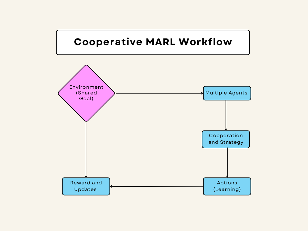
Diagram: Cooperative MARL Workflow

Here is a detailed visual representation of how cooperative MARL works:

Real-World Applications of Reinforcement Learning

Reinforcement Learning in Healthcare

Personalized Treatment Plans

Reinforcement learning (RL) can be a powerful tool in healthcare, especially for creating personalized treatment plans for patients. This approach allows treatment strategies to be adapted based on each patient’s unique health data, aiming to improve outcomes more effectively than traditional methods.

Key Aspects:

• Dynamic Adaptation: RL models can continuously modify treatment plans based on how the patient is responding over time. This means that as new data comes in, the RL model can adjust the treatment to better fit the patient’s current condition.
• Individualization: RL uses detailed, patient-specific information such as medical history and genetic data. This helps in tailoring the treatment to fit each patient’s unique needs.

Example:

For managing chronic conditions like diabetes, an RL model can adjust insulin dosages based on real-time glucose readings. This helps in optimizing long-term health outcomes by ensuring that insulin levels are adjusted to match current glucose levels.

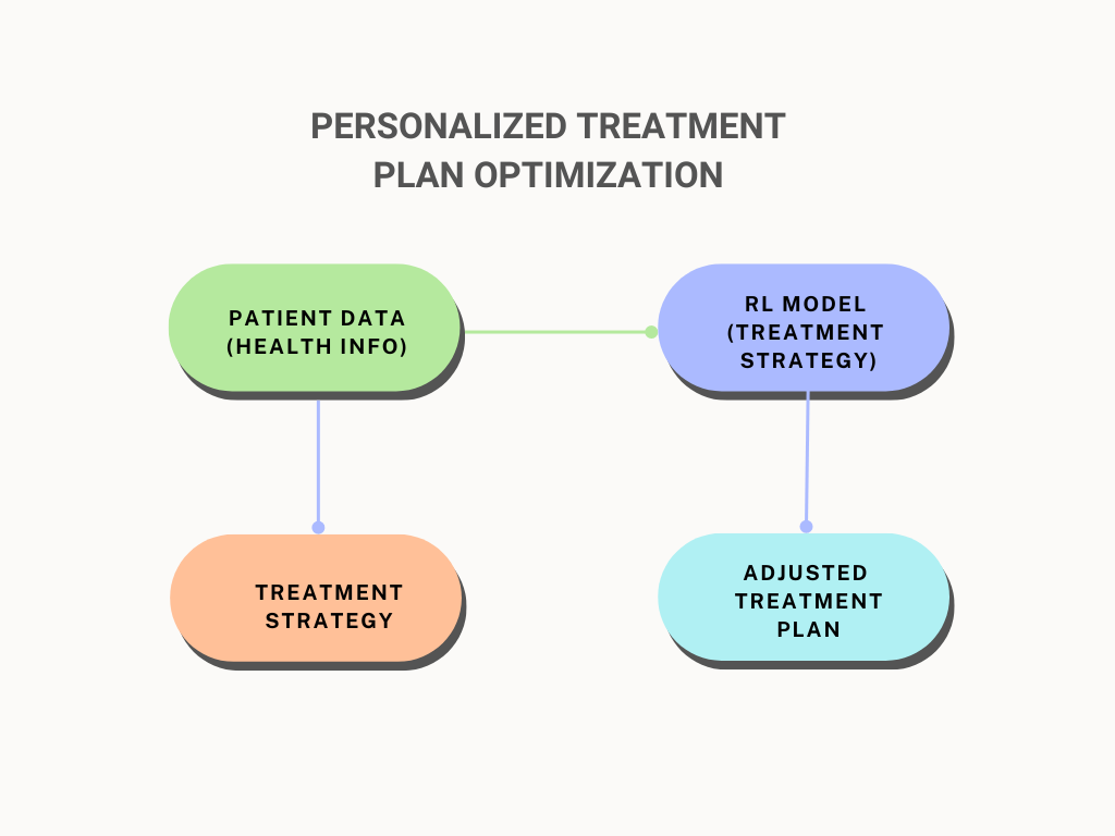
Diagram 1: Personalized Treatment Plan Optimization

This diagram illustrates how RL can be used to optimize personalized treatment plans:

• Patient Data: The model starts with data about the patient’s health, including medical history and current health metrics.
• RL Model: This data is fed into the RL model, which uses it to generate a treatment strategy tailored to the patient’s needs.
• Adjusted Treatment Plan: Based on the RL model’s recommendations, the treatment plan is updated to better suit the patient’s current condition.

Example Code:

Here’s a simple example of how an RL agent might adjust treatment plans using a Q-learning approach:

import numpy as np

# Define the RL agent for treatment adjustment
class TreatmentAgent:
    def __init__(self, num_states, num_actions):
        self.q_table = np.zeros((num_states, num_actions))  # Initialize Q-table

    def choose_action(self, state):
        return np.argmax(self.q_table[state])  # Choose the action with highest Q-value

    def update_q_table(self, state, action, reward, next_state, alpha, gamma):
        best_next_action = np.argmax(self.q_table[next_state])
        td_target = reward + gamma * self.q_table[next_state, best_next_action]
        td_error = td_target - self.q_table[state, action]
        self.q_table[state, action] += alpha * td_error

# Example usage
num_states = 10  # Number of possible states (e.g., different health conditions)
num_actions = 3  # Number of possible treatment actions (e.g., different dosages)
agent = TreatmentAgent(num_states, num_actions)

# Print the initial Q-table
print("Initial Q-table:")
print(agent.q_table)

# Simulate an action and update
state = 0
action = agent.choose_action(state)
reward = 1  # Example reward
next_state = 1
alpha = 0.1
gamma = 0.9

print(f"Chosen action: {action}")

agent.update_q_table(state, action, reward, next_state, alpha, gamma)

# Print the updated Q-table
print("Updated Q-table:")
print(agent.q_table)

• Initialization: The agent starts with a Q-table, which stores the expected rewards for each action in each state.
• Choosing Actions: The agent selects actions based on the highest value in the Q-table for the current state.
• Updating Q-Table: After taking an action and receiving feedback (reward), the Q-table is updated to reflect the new knowledge, helping the agent make better decisions in the future.

This RL approach helps in creating more effective and personalized treatment plans by continuously learning from new data.

Output

Initial Q-table:

[[0. 0. 0.]
 [0. 0. 0.]
 [0. 0. 0.]
 [0. 0. 0.]
 [0. 0. 0.]
 [0. 0. 0.]
 [0. 0. 0.]
 [0. 0. 0.]
 [0. 0. 0.]
 [0. 0. 0.]]

This shows that the Q-table is initialized with zeros, which is what you’d expect at the beginning.

Chosen action: 0 This indicates that the action chosen by the agent for state 0 is action 0. This is because all Q-values are initially zero, so np.argmax will always return 0.

Updated Q-table:

[[0.1 0.  0. ]
 [0.  0.  0. ]
 [0.  0.  0. ]
 [0.  0.  0. ]
 [0.  0.  0. ]
 [0.  0.  0. ]
 [0.  0.  0. ]
 [0.  0.  0. ]
 [0.  0.  0. ]
 [0.  0.  0. ]]

The Q-value for state 0 and action 0 has been updated from 0 to 0.1, reflecting the reward you provided and the learning rate (alpha).

Reinforcement Learning for Financial Modeling

Stock Market Prediction

Reinforcement Learning (RL) is a powerful tool for forecasting stock prices and making trading decisions. The core idea is to train a model that learns to make the best trading decisions based on historical and real-time market data. Here’s a more detailed look at how RL is applied in this context:

Key Aspects

1. Dynamic Strategies:
   • Adaptive Learning: RL models are designed to adjust their strategies dynamically. This means they can update their approach based on new data and changing market conditions.
   • Continuous Improvement: As the model interacts with the market, it continually learns and refines its strategies to improve performance over time.
2. Risk Management:
   • Loss Minimization: RL can incorporate strategies to minimize potential losses. For example, it might learn to avoid risky trades or set stop-loss orders to protect against significant losses.
   • Balanced Approach: The model can balance between risk and return, optimizing strategies not just for profit but also for risk mitigation.

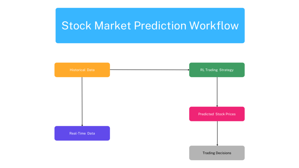
Diagram 3: Stock Market Prediction Workflow

Here’s a step-by-step workflow of how RL is used for stock market prediction:

1. Historical Data:
   • What It Is: This data includes past stock prices, trading volumes, and other relevant financial indicators.
   • Purpose: The RL model uses this historical data to understand trends and patterns in the stock market.
2. RL Trading Strategy:
   • Training: The model uses the historical data to train itself. It learns to make decisions based on this data to optimize trading strategies.
   • Adjustment: As the model learns, it adjusts its strategies to improve its predictions and trading decisions.
3. Predicted Stock Prices:
   • Forecasting: The RL model predicts future stock prices based on its training. These predictions help in making trading decisions.
4. Real-Time Data:
   • What It Is: This includes current stock prices and market conditions.
   • Purpose: The model uses real-time data to update its predictions and adjust its trading strategy accordingly.
5. Trading Decisions:
   • Action: Based on predicted stock prices and real-time data, the model makes decisions such as buying, selling, or holding stocks.
   • Optimization: These decisions aim to maximize returns while managing risk.

Example Code

Here’s a simple example of setting up an RL environment for stock trading using Python and the Gym library:

import gym
import numpy as np

# Define the RL environment for stock trading
class StockTradingEnv(gym.Env):
    def __init__(self):
        super(StockTradingEnv, self).__init__()
        self.action_space = gym.spaces.Discrete(num_actions)  # Possible actions: Buy, Sell, Hold
        self.observation_space = gym.spaces.Box(low=-np.inf, high=np.inf, shape=(num_features,))
        self.state = np.zeros(num_features)  # Initialize state
        
    def reset(self):
        # Reset the environment to an initial state
        self.state = np.zeros(num_features)
        print("Environment reset.")
        return self.state

    def step(self, action):
        # Apply the chosen action and return the new state, reward, and done flag
        print(f"Action taken: {action}")
        reward = 0  # Placeholder for reward
        done = False  # Placeholder for done flag
        self.state = np.random.randn(num_features)  # Example new state
        return self.state, reward, done, {}

# Example usage
num_actions = 3  # Actions: Buy, Sell, Hold
num_features = 10  # Number of features in the state representation

env = StockTradingEnv()

# Test the environment
state = env.reset()
print(f"Initial state: {state}")

action = env.action_space.sample()  # Random action
next_state, reward, done, _ = env.step(action)
print(f"Next state: {next_state}, Reward: {reward}, Done: {done}")

1. StockTradingEnv Class:
   • Purpose: This class defines the environment where the RL model will operate. It sets up the action and observation spaces.
   • Action Space: This specifies the possible actions the model can take, such as buying, selling, or holding stocks.
   • Observation Space: This defines the features of the state, such as stock prices and other financial indicators.
2. reset Method:
   • Function: This method resets the environment to its initial state at the start of each episode. This is necessary to begin a new round of trading.
3. step Method:
   • Function: This method applies the chosen action (buy, sell, or hold) and returns the updated state of the environment, the reward received for the action, and whether the episode is complete.

By setting up an RL environment like this, you can train models to make trading decisions based on historical and real-time data, aiming to optimize trading strategies and improve financial outcomes.

Output

Environment Reset:

Environment reset.
Initial state: [0. 0. 0. 0. 0. 0. 0. 0. 0. 0.]

This confirms that the environment resets correctly, initializing the state to an array of zeros.

Action Taken:

Action taken: 2

This shows that a random action (2, which corresponds to Hold in your setup) was chosen and executed.

Next State:

Next state: [ 8.76561919e-01 -8.63979588e-01 -2.41873354e-03 -2.85826601e+00
-1.44343463e+00 -1.38290353e+00 -8.70951965e-01  2.23898453e+00
-2.39560145e-01 -1.03687550e-02]

This shows the new state after the action was taken. The state is randomly generated in this placeholder implementation.

Reward and Done Flag:

Reward: 0, Done: False

1. Since you are using placeholders, the reward is 0 and done is False, indicating that the episode hasn’t ended.

Next Steps:

1. Implement Real Logic: Replace placeholder logic in reset and step methods with actual stock trading logic, including calculating rewards and determining when an episode should end.
2. Enhance Testing: Expand the testing code to include different actions, longer episodes, and additional logging to observe the environment’s behavior over time.
3. Integrate with RL Algorithms: Connect this environment with a reinforcement learning algorithm to train an agent and evaluate its performance.

Challenges and Future Directions in Reinforcement Learning

Reinforcement Learning (RL) has made significant progress, but several challenges remain that need to be addressed for the field to advance further. Additionally, future directions in RL offer promising opportunities to enhance its capabilities. This article explores both the current challenges and potential future developments in RL.

Challenges in Reinforcement Learning

Data Efficiency and Scalability

Data efficiency refers to the ability of RL algorithms to learn effectively with limited data. Scalability involves the capacity of these algorithms to handle increasingly complex environments and larger datasets.

Key Issues:

• High Sample Complexity: Many RL algorithms require a large number of interactions with the environment to learn effectively, which can be computationally expensive and time-consuming.
• Scalability: As environments become more complex, such as with high-dimensional state and action spaces, the computational resources required to train RL models increase significantly.

Example: Training an RL model to play a video game might require millions of game frames to achieve optimal performance. This is impractical for real-world applications where collecting such extensive data is challenging.

Exploration vs. Exploitation Dilemma

The exploration vs. exploitation dilemma is a fundamental challenge in RL. It involves finding a balance between exploring new actions to discover better strategies (exploration) and exploiting known strategies that provide high rewards (exploitation).

Key Issues:

• Over-Exploration: Excessive exploration can lead to inefficient learning, where the agent spends too much time trying out suboptimal actions.
• Over-Exploitation: Excessive exploitation can result in suboptimal performance if the agent fails to discover better actions.

Example: In a robot learning to navigate a maze, too much exploration might lead it to repeatedly explore dead ends, while too much exploitation might prevent it from discovering shorter paths.

Ethical Considerations and Bias in RL Models

Ethical considerations and bias are critical issues in RL. Biases in RL models can arise from biased training data or flawed reward structures, leading to unfair or unethical outcomes.

Key Issues:

• Bias in Training Data: If the data used to train RL models contains biases, the model may replicate and even exacerbate these biases.
• Unintended Consequences: Poorly designed reward functions can lead to unintended and potentially harmful behavior.

Example: A recommendation system trained with biased data might recommend products based on biased preferences, leading to discrimination against certain user groups.

Future Directions in Reinforcement Learning

Advancements in Hierarchical RL

Hierarchical Reinforcement Learning (HRL) involves breaking down complex tasks into simpler, more manageable sub-tasks. This approach helps in solving problems that are too difficult to handle in a flat, single-level RL setting.

Key Aspects:

• Decomposition: HRL decomposes tasks into a hierarchy of sub-tasks, each with its own set of goals and rewards.
• Modularity: HRL improves modularity by separating high-level decision-making from low-level control.

Example: In a robot learning to cook, HRL can decompose the task into high-level goals (e.g., prepare a meal) and sub-tasks (e.g., chop vegetables, boil water).

Meta-Reinforcement Learning

Meta-Reinforcement Learning aims to develop RL models that can adapt quickly to new tasks with minimal additional training. This approach focuses on learning how to learn, enabling models to generalize across a variety of tasks.

Key Aspects:

• Few-Shot Learning: Meta-RL models are designed to perform well even with limited data for new tasks.
• Adaptability: Models can rapidly adapt to changes in the environment or task requirements.

Example: A meta-RL model trained on various navigation tasks could quickly adapt to new environments with minimal additional training.

Integration with Other AI Techniques

Integration with other AI techniques involves combining RL with approaches from other areas of AI, such as supervised learning and unsupervised learning, to enhance performance and capabilities.

Key Aspects:

• Hybrid Models: Combining RL with supervised learning can improve the efficiency of training and generalization.
• Multi-Modal Learning: Integrating RL with unsupervised learning can enable models to learn from diverse types of data.

Example: A hybrid model combining RL with supervised learning can use labeled data to guide exploration in environments where obtaining rewards is challenging.

Conclusion

Reinforcement Learning (RL) is rapidly advancing and transforming how we approach complex decision-making tasks. The future of RL promises even more significant breakthroughs and applications across various industries. This conclusion summarizes key points, explores the potential impact of RL, and encourages further research and innovation.

Summary of Key Points

Reinforcement Learning has evolved considerably, addressing complex challenges and opening new avenues for research and application. Here are some key points to consider:

• Data Efficiency and Scalability: RL models face challenges related to high sample complexity and the need for scalable solutions. Techniques like experience replay and simulated environments are helping to address these issues.
• Exploration vs. Exploitation: Balancing exploration and exploitation is critical for effective learning. Approaches like the ε-greedy policy help in managing this balance.
• Ethical Considerations: Bias and fairness are crucial concerns in RL. Implementing fairness constraints and bias detection mechanisms is essential to ensure ethical outcomes.
• Future Directions: Advancements in Hierarchical RL, Meta-RL, and integration with other AI techniques are promising directions that can enhance RL’s capabilities and applications.

The Potential Impact of RL on Various Industries

Reinforcement Learning has the potential to revolutionize several industries by optimizing complex systems and improving decision-making processes. Below are examples of how RL could impact various sectors:

• Healthcare: RL can personalize treatment plans and accelerate drug discovery by optimizing experimental designs and predicting treatment outcomes.
• Finance: In the financial sector, RL models can enhance stock market prediction accuracy and automate trading strategies to maximize returns.
• Autonomous Vehicles: RL enables advancements in self-driving car technologies and traffic management solutions, improving road safety and efficiency.

Encouraging Further Research and Innovation

To fully realize the potential of Reinforcement Learning, continued research and innovation are essential. Several areas are ripe for exploration:

• Algorithmic Improvements: Enhancing existing algorithms for better performance, efficiency, and scalability.
• Real-World Applications: Expanding RL applications to new domains and real-world problems.
• Ethical and Fairness Considerations: Developing robust methods to address bias and ensure fairness in RL models.

Researchers, practitioners, and organizations should collaborate to advance RL technologies and address the challenges outlined. Investment in research and development, coupled with interdisciplinary efforts, will drive progress and unlock new possibilities.

Conclusion

Reinforcement Learning continues to be a transformative technology with broad applications and significant potential for future advancements. By addressing current challenges and exploring new research directions, RL can drive innovation and bring substantial benefits across various industries. The collaborative efforts of researchers, practitioners, and policymakers will be crucial in shaping the future of RL and ensuring its responsible and effective deployment.

FAQs

External Resources

1. Deep Reinforcement Learning: An Overview
   A comprehensive survey of recent advancements and research in deep reinforcement learning, covering key algorithms, applications, and challenges.
2. Proximal Policy Optimization Algorithms
   The original paper introducing Proximal Policy Optimization (PPO), detailing the algorithm and its improvements over previous methods.
3. Playing Atari with Deep Reinforcement Learning
   The seminal paper on Deep Q-Networks (DQN), which explores the use of deep learning techniques for reinforcement learning in complex environments.
4. Asynchronous Methods for Deep Reinforcement Learning
   The paper on Asynchronous Actor-Critic Agents (A3C), describing the algorithm’s architecture and benefits for training reinforcement learning agents.
5. Multi-Agent Reinforcement Learning: A Review
   A review of multi-agent reinforcement learning, discussing the challenges, advancements, and future directions in this area.

About The Author

Emmimal Alexander

Welcome! I’m Emmimal Alexander, a trailblazer in the tech world with a unique background that bridges business and technology. As an Anna University Rank Holder, I hold a Master’s in Business Administration and a Bachelor’s in Computer Applications. My career began in the corporate world as an HR executive, then shifted to NSE trading, and finally led me to specialize in artificial intelligence, machine learning, deep learning, and programming languages like Python, HTML, JavaScript, and CSS.

Now, as the founder of EmitechLogic, I’m dedicated to empowering others to master the complexities of AI, ML, DL, and programming. My passion for technology and creative expression drives me to make these advanced fields accessible, practical, and engaging for learners of all levels. Through EmitechLogic, I provide insightful resources, tutorials, and discussions that help professionals and enthusiasts stay ahead in the rapidly evolving tech landscape.

Throughout my journey, I’ve worked on exciting projects like synthetic data generation, neural networks, and creative writing. My mission is to inspire curiosity, share knowledge, and foster a deeper understanding of the endless possibilities technology offers.

When I’m not writing or experimenting with new tech, you’ll find me enjoying creative projects or the beauty of nature. I invite you to explore my blog, connect through my experiences, and join me as we uncover the limitless potential of AI and innovation together!

See author's posts