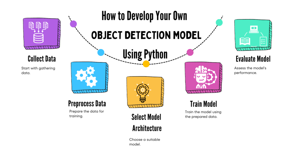
How to Develop Your Own Object Detection Model Using Python
Introduction
Imagine a world where technology doesn’t just respond to commands but understands its surroundings like a human would. That’s the magic of object detection. This cutting-edge technology is revolutionizing how machines perceive and interact with the world, making it a cornerstone of modern innovation.
From autonomous vehicles that navigate busy streets by recognizing other cars, pedestrians, and road signs, to smart home devices that can differentiate between family members and strangers, object detection is everywhere. It’s the unseen hero behind a range of applications that impact our daily lives, making technology smarter and more intuitive.
In this blog post, we’ll journey through the fascinating world of object detection. We’ll uncover what it is, why it’s crucial for the technologies we use every day, and how it’s shaping the future. Plus, by the end of this article, you’ll be able to create your own object detection app using Python. Get ready to see how this remarkable technology is not just enhancing, but transforming the way we interact with the digital world.
What is Object Detection?
Object detection is a powerful computer vision technology that allows machines to not only identify objects in images or videos but also find their exact location. Think of it as a system that can spot a dog in a photo or pick out a traffic sign in a video. It’s like giving machines the ability to see and understand what’s around them.
Definition and Significance
In simple terms, object detection involves two main tasks: figuring out what an object is and pinpointing where it is. This is done by drawing bounding boxes around objects and labeling them. For instance, a security camera using object detection might recognize and mark a person, a car, and a bicycle in its feed. This technology is crucial in many areas, from self-driving cars that need to recognize and react to their environment, to smart home systems that differentiate between different people or objects. It makes technology smarter and more capable of interacting with the real world.
Differences Between Object Detection, Recognition, and Classification
While object detection, recognition, and classification are all related, they do different things:
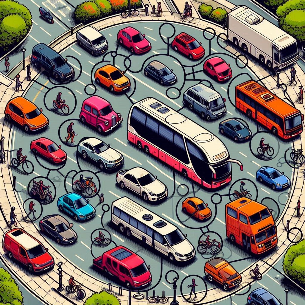
Object Detection: Finds and identifies objects in an image or video, and shows where they are by drawing boxes around them. For example, it would detect all the cars, bicycles, and people in a street scene.
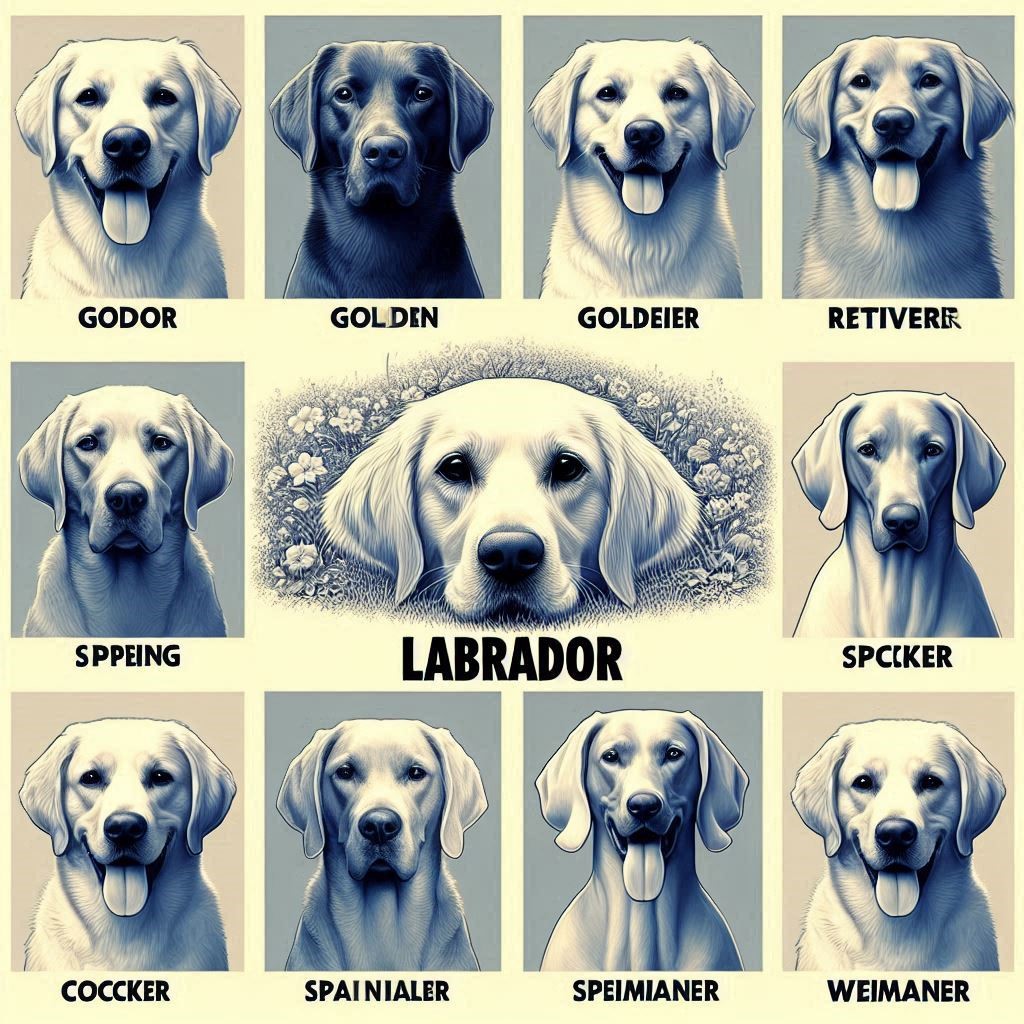
Object Recognition: Takes it a step further by identifying exactly what each object is. For instance, it can recognize that a dog is a Labrador. Recognition often comes after detection, adding more detail about each object.
Object Classification: Categorizes objects into broad groups. It tells you if something is a cat, a dog, or a car, but doesn’t locate it within the image. Classification usually happens before detection and recognition.
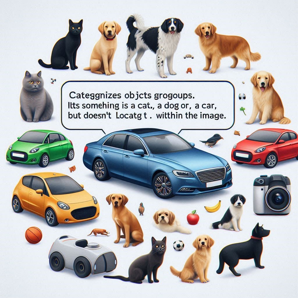
Understanding these differences helps clarify how they all work together to make technology more effective and responsive.
Prerequisites for Developing an Object Detection Model
If you’re interested in developing an object detection model, there are a few essential prerequisites you’ll need to get started. Let’s break them down into two main areas: programming basics and the tools you’ll use.
Python Programming Basics
Python is a versatile and beginner-friendly programming language that’s widely used in the field of machine learning and computer vision. It’s popular because of its simple syntax, readability, and a vast ecosystem of libraries and frameworks. If you’re new to Python, you’ll want to get comfortable with basic programming concepts like variables, loops, and functions. These fundamentals will help you navigate and implement object detection models more effectively.
Why Python is Popular for Machine Learning and Computer Vision
Python’s popularity in machine learning and computer vision comes from its ease of use and the extensive support it offers through various libraries and frameworks. Its rich ecosystem allows you to focus on solving problems rather than dealing with complex programming details. Libraries such as TensorFlow and Keras provide powerful tools for building and training models, while OpenCV helps with image processing tasks. Python’s community support also means that you’ll find plenty of resources and tutorials to help you along the way.
Libraries and Tools
To build an object detection model, you’ll need to get familiar with a few key libraries and tools:
- TensorFlow: An open-source framework developed by Google, TensorFlow is used for building and training machine learning models. It offers extensive support for various neural networks and deep learning techniques, making it a cornerstone for many object detection projects.
- Keras: Keras is a high-level API that runs on top of TensorFlow. It simplifies the process of building and training neural networks with an easy-to-use interface. Keras is ideal for quickly prototyping and experimenting with different model architectures.
- OpenCV: Short for Open Source Computer Vision Library, OpenCV is a powerful tool for image and video processing. It’s widely used for real-time computer vision tasks and provides functions for manipulating images, detecting features, and more.
- NumPy: A fundamental package for scientific computing with Python, NumPy is used for handling arrays and performing numerical operations. It’s essential for manipulating image data and performing computations in your object detection pipeline.
Must Read
- Machine Learning Model Deployment: How to Deploy a Machine Learning Model to Production (Step-by-Step)
- Machine Learning Production Pipeline: Complete System Design Guide
- How to Detect and Fix Production Drift in Machine Learning (Complete Guide)
- How to Diagnose and Fix Class Imbalance in Machine Learning (Complete Guide)
- How to Diagnose Overfitting in Machine Learning — 9 Proven Tools
Installation Guide for Required Libraries
Here’s a step-by-step guide to installing the necessary libraries:
- Install Python:
- Go to the official Python website and download the latest version of Python.
- Follow the installation instructions for your operating system (Windows, macOS, or Linux).
- Verify Python Installation:
- Open your command line or terminal and type:
python --version
- You should see the version number of Python, confirming the installation was successful.
3. Install Pip:
- Check if pip (Python’s package installer) is installed by typing:
pip --version
If it’s not installed, follow the instructions here.
4. Install Required Libraries:
- Use pip to install the libraries by typing:
pip install tensorflow keras opencv-python numpy
Setting Up Your Environment
To maintain an organized and conflict-free workspace, it’s recommended to set up a virtual environment.
Benefits of Using Virtual Environments
- Isolation: Each project can have its own set of dependencies without interfering with others.
- Version Control: You can manage different versions of libraries for different projects.
- Cleaner Workspace: Keeps your global Python environment clean and uncluttered.
How to Create and Activate a Virtual Environment
- Install Virtual Environment Package:
- If you don’t have the
venvmodule, you can install it by running:
- If you don’t have the
pip install virtualenv
2. Create a Virtual Environment:
- Navigate to your project directory in the command line or terminal.
- Create a virtual environment by typing:
python -m venv myenv
- Replace
myenvwith your preferred name for the environment.
3. Activate the Virtual Environment:
- For Windows:
myenv\Scripts\activate
- For macOS and Linux:
source myenv/bin/activate
- You’ll see the name of your virtual environment in the command prompt, indicating that it’s active.
4. Install Required Libraries in the Virtual Environment:
- With the virtual environment activated, install the libraries:
pip install tensorflow keras opencv-python numpy
5. Deactivate the Virtual Environment:
- When you’re done working in the virtual environment, deactivate it by typing:
deactivate
By following these steps, you’ll set up a solid foundation for developing your object detection model, ensuring you have all the necessary tools and a clean, organized workspace.
Understanding the Dataset for Object Detection
To build an effective object detection model, choosing and preparing the right dataset is crucial. Think of the dataset as the material your model learns from. Here’s a step-by-step guide to selecting and annotating a dataset.
Choosing a Dataset for Object Detection
Selecting the right dataset is the first step in creating a successful object detection model. Here’s a look at some popular options:
Popular Datasets
- COCO (Common Objects in Context):
- Overview: COCO is a large dataset with over 330,000 images. It covers 80 different object categories, like people, cars, and animals. Each image is annotated with details like bounding boxes, segmentation masks, and keypoints.
- Best For: This dataset is great for training models to recognize a variety of everyday objects in different environments.
- How to Access: You can download the dataset from the COCO website, which provides all the data and documentation you need.
- PASCAL VOC (Visual Object Classes):
- Overview: The PASCAL VOC dataset includes images of 20 object categories, such as cats, dogs, and birds. It offers bounding boxes around objects, making it simpler compared to COCO.
- Best For: This is a good option if you’re focusing on a specific set of objects and need straightforward annotations.
- How to Access: Download it from the PASCAL VOC website, where you’ll find the dataset and guidelines.
- ImageNet:
- Overview: ImageNet is a large visual database with over 14 million images across thousands of categories. It’s commonly used for image classification but can also be used for object detection.
- Best For: Ideal if you need a broad range of object categories and a large amount of data.
- How to Access: Visit the ImageNet website to explore and request access to the dataset.
Annotating the Dataset for Object Detection
Once you have your dataset, you might need to add annotations if they’re not already included. Annotations are labels that indicate what’s in the image and where it’s located. Here’s how to handle this process:
Tools for Image Annotation
- LabelImg:
- Overview: LabelImg is a user-friendly tool for creating bounding boxes and labeling objects in images. It supports formats like Pascal VOC and YOLO, which are used in object detection.
- Features: Allows you to draw boxes around objects and save these annotations in XML (Pascal VOC) or TXT (YOLO) formats.
- How to Install: Install LabelImg via GitHub or pip. To install via pip, run:
pip install labelImg
- How to Use: Open LabelImg, load your images, and draw bounding boxes around objects. The tool makes it easy to manage and save your annotations.
- Website: Visit LabelImg on GitHub for more details and installation instructions.
Best Practices for Annotating Images for Object Detection
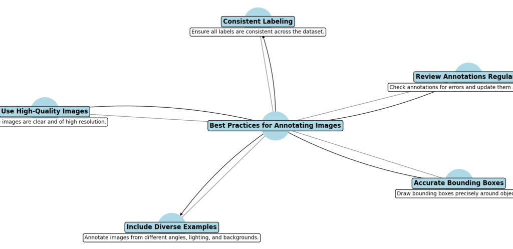
- Be Consistent:
- Consistent annotations are essential. Ensure that objects of the same type are labeled similarly throughout your dataset. For instance, use the same bounding box format and size for cars in all images.
- Accuracy Matters:
- Make sure your bounding boxes or segmentation masks fit closely around the objects without including too much background or cutting off parts of the object. Accurate annotations help your model learn better.
- Clear Labels:
- Each label should accurately describe the object. If your dataset includes various categories, ensure that each object is labeled according to its correct category.
- Diverse Examples:
- Include images that show objects in different environments, lighting conditions, and angles. This variety helps your model learn to detect objects in a wide range of scenarios.
- Review and Check:
- After annotating, review your work to correct any mistakes or inconsistencies. This helps maintain the quality of your dataset and ensures your model gets reliable training data.
By carefully choosing and annotating your dataset, you provide your object detection model with the high-quality data it needs to learn and perform well. This solid foundation will help your model accurately identify and locate objects.
Preprocessing the Data for Object Detection model
Before you train your object detection model, you need to prepare your data. This involves augmenting the data to make it more diverse and splitting it into different sets for training and evaluation. Here’s a detailed look at these steps:
Data Augmentation Techniques
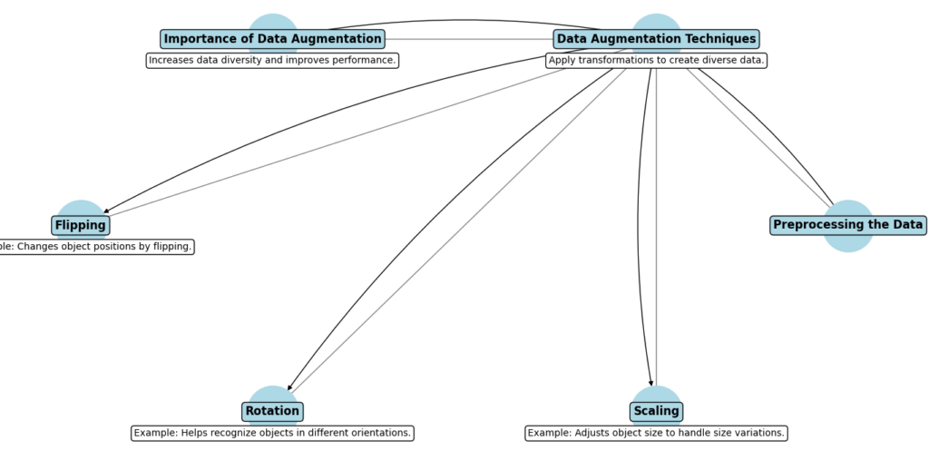
Data augmentation is a technique used to increase the variety of your training data by applying different transformations. This helps your model learn to handle various scenarios and improves its performance. Here’s why data augmentation is important and some common techniques:
Importance of Data Augmentation
- Increases Data Diversity: By transforming your images, you create new variations of the data. This helps the model generalize better by learning from a more diverse set of examples.
- Improves Model Performance: More varied training data can lead to better performance because the model learns to recognize objects under different conditions.
Common Techniques
- Flipping: This involves flipping images horizontally or vertically. It’s useful for making the model learn to recognize objects from different perspectives.
- Example: If an object appears on the left side of an image, flipping it will place it on the right side, helping the model handle different orientations.
- Rotation: Rotating images by various angles can help the model learn to detect objects regardless of their orientation.
- Example: Rotating an image by 90 degrees can teach the model to recognize objects in portrait or landscape modes.
- Scaling: Scaling changes the size of objects in images. This helps the model learn to detect objects that appear larger or smaller in different images.
- Example: Scaling an object up or down helps the model handle variations in object size.
Preparing Data for Training
Once you have augmented your data, the next step is to prepare it for training. This involves splitting the dataset and formatting it for use with machine learning libraries like TensorFlow/Keras.
Splitting the Dataset
To evaluate the performance of your model effectively, you need to divide your data into three main sets:
- Training Set: This is the largest portion of your data, used to train the model. The model learns to detect and classify objects from this set.
- Validation Set: This set is used during training to tune the model’s hyperparameters and make adjustments. It helps you monitor the model’s performance and make improvements.
- Test Set: This is a separate portion of data used to evaluate the final performance of your model. It helps determine how well the model performs on new, unseen data.
Loading and Formatting the Data Using TensorFlow/Keras
You’ll need to load and preprocess your data so it’s ready for training with TensorFlow/Keras. Here’s an example of how you might do this in Python:
import tensorflow as tf

# Example function to load and preprocess data
def load_and_preprocess_data(dataset_path):
    # Load the dataset
    dataset = tf.data.Dataset.list_files(dataset_path + '/*.jpg')

    # Define a function to parse and preprocess each image
    def preprocess_image(file_path):
        # Load image from file
        image = tf.io.read_file(file_path)
        image = tf.image.decode_jpeg(image, channels=3)

        # Resize image to desired size
        image = tf.image.resize(image, [224, 224])

        # Normalize image
        image = image / 255.0

        return image

    # Apply preprocessing to each image
    dataset = dataset.map(preprocess_image)

    # Split dataset into training, validation, and test sets
    train_size = int(0.8 * len(dataset))
    val_size = int(0.1 * len(dataset))
    test_size = len(dataset) - train_size - val_size

    train_data = dataset.take(train_size)
    val_data = dataset.skip(train_size).take(val_size)
    test_data = dataset.skip(train_size + val_size)

    return train_data, val_data, test_data
Breakdown of the Code
- Import TensorFlow: The code starts by importing the TensorFlow library, which is essential for handling the data and building models.
- Load the Dataset:
dataset = tf.data.Dataset.list_files(dataset_path + '/*.jpg')
This line creates a dataset consisting of file paths for all .jpg images in the specified directory. The dataset_path variable should point to the location of your images.
3. Define a Preprocessing Function:
def preprocess_image(file_path):
    image = tf.io.read_file(file_path)
    image = tf.image.decode_jpeg(image, channels=3)
    image = tf.image.resize(image, [224, 224])
    image = image / 255.0
    return image
This function performs several steps:
- Read the image file:
tf.io.read_file(file_path)loads the raw image data from the file. - Decode the image:
tf.image.decode_jpeg(image, channels=3)converts the raw data into an image tensor with three color channels (RGB). - Resize the image:
tf.image.resize(image, [224, 224])changes the image dimensions to 224×224 pixels, which is a common size for model input. - Normalize the image:
image / 255.0scales pixel values to a range of 0 to 1, which helps the model learn better.
4. Apply Preprocessing:
dataset = dataset.map(preprocess_image)
The map function applies the preprocess_image function to each image in the dataset, transforming all images as specified.
5. Split the Dataset:
train_size = int(0.8 * len(dataset))
val_size = int(0.1 * len(dataset))
test_size = len(dataset) - train_size - val_size

train_data = dataset.take(train_size)
val_data = dataset.skip(train_size).take(val_size)
test_data = dataset.skip(train_size + val_size)
- Calculate sizes: The dataset is divided into training (80%), validation (10%), and test sets (10%).
- Create subsets:
take(train_size)retrieves the first portion of the dataset for training.skip(train_size).take(val_size)gets the next portion for validation.skip(train_size + val_size)gets the remaining data for testing.
6. Return Data: The function returns the three datasets: train_data, val_data, and test_data, which are now ready for training, validating, and testing your model.
By following these steps, you ensure that your object detection model is trained on a diverse and well-prepared dataset, improving its ability to detect and classify objects accurately.
Building the Object Detection Model
Choosing the right architecture for your object detection model is crucial as it determines how well your model will perform. Here’s a more detailed explanation of some popular architectures used in object detection:
Choosing the Right Architecture
Different object detection architectures have their unique strengths and weaknesses. Here’s an in-depth look at three widely used architectures:
YOLO (You Only Look Once)
Overview:
- YOLO is renowned for its speed. It processes the entire image in a single forward pass through the network. This approach makes it incredibly fast compared to other object detection models.
- The model divides the image into a grid and, for each grid cell, predicts bounding boxes and class probabilities simultaneously.
Strengths:
- Speed: YOLO’s single-stage detection process allows it to analyze images in real-time, making it ideal for applications where quick responses are needed, such as live video analysis or real-time object tracking.
- Efficiency: Because YOLO handles the entire image at once, it reduces computational overhead and simplifies the detection pipeline.
Weaknesses:
- Accuracy for Small Objects: YOLO’s grid-based approach can limit its ability to accurately detect small objects. Each grid cell only predicts a fixed number of boxes and classes, which might not capture smaller objects well.
- Localization: The bounding box predictions can sometimes be less precise due to the grid cell constraints, leading to less accurate object localization.
Applications:
- Ideal for scenarios where speed is more critical than pinpoint accuracy, such as in real-time surveillance systems or autonomous vehicles.
SSD (Single Shot MultiBox Detector)
Overview:
- SSD combines speed and accuracy by using multiple feature maps at different scales to detect objects. It predicts bounding boxes and class scores for each feature map, allowing the model to handle objects of various sizes.
- Unlike YOLO, SSD uses a series of convolutional layers to detect objects at multiple scales, which helps it better detect objects of different sizes and aspect ratios.
Strengths:
- Balance of Speed and Accuracy: SSD provides a good compromise between fast processing and accurate object detection. It’s faster than models like Faster R-CNN while still delivering reliable performance.
- Multi-scale Detection: The use of feature maps at different scales improves the model’s ability to detect objects of varying sizes, which is beneficial for a range of applications.
Weaknesses:
- Not as Precise as Faster R-CNN: While SSD is effective, it might not be as accurate as Faster R-CNN in some scenarios, particularly when detecting small or overlapping objects.
- Trade-off: The balance between speed and accuracy might not be ideal for applications that require extremely high precision.
Applications:
- Suitable for applications where a good balance between speed and accuracy is needed, such as object detection in mobile devices or real-time video analysis.
Faster R-CNN (Region-based Convolutional Neural Networks)
Overview:
- Faster R-CNN is known for its high accuracy. It uses a two-stage process: first, a Region Proposal Network (RPN) generates region proposals, then a separate network refines these proposals and classifies the objects within them.
- The RPN suggests regions of interest where objects might be, and the second stage refines these regions to improve accuracy and classify the objects.
Strengths:
- High Accuracy: The two-stage approach allows Faster R-CNN to achieve high accuracy in object detection by focusing on potential object regions and refining predictions.
- Detailed Object Detection: It excels at handling complex scenes and detecting objects with high precision, which is beneficial for tasks requiring fine-grained detection.
Weaknesses:
- Slower Speed: The two-stage process involves additional computation, making Faster R-CNN slower compared to single-stage models like YOLO and SSD. This might not be suitable for applications requiring real-time detection.
- Complexity: The model’s complexity can make it more challenging to implement and train compared to simpler architectures.
Applications:
- Best suited for applications where accuracy is more important than speed, such as detailed image analysis or medical imaging where precise object detection is critical.
Implementing the Object Detection Model in Python
Now that we’ve installed the required libraries and set up our virtual environment, let’s import everything we need to build our object detection model.
Import Necessary Libraries
Create a Python script, object_detection_model.py, and import the required libraries:
import tensorflow as tf
import numpy as np
import os
import six.moves.urllib as urllib
import sys
import tarfile
import zipfile
import pathlib
import pandas as pd
import cv2
import matplotlib.pyplot as plt
from collections import defaultdict
from io import StringIO
from matplotlib import pyplot as plt
from IPython.display import display
from IPython.display import Image
from sklearn.model_selection import train_test_split
Explanation:
- These imports bring in necessary libraries and modules for handling data, downloading files, image processing, and model interaction.
tensorflow: For building and running the object detection model.numpy: For numerical operations, particularly with image arrays.cv2: OpenCV library for image processing.matplotlib.pyplot: For visualizing images and results.
2. Define Model URL and Download It
# Define the model URL and download it
MODEL_NAME = 'ssd_mobilenet_v2_fpnlite_320x320'
BASE_URL = 'http://download.tensorflow.org/models/object_detection/'
MODEL_FILE = MODEL_NAME + '.tar.gz'
PATH_TO_MODEL_DIR = 'models'
PATH_TO_FROZEN_GRAPH = PATH_TO_MODEL_DIR + '/' + MODEL_NAME + '/frozen_inference_graph.pb'

# Download and extract the model
if not pathlib.Path(PATH_TO_MODEL_DIR).exists():
    pathlib.Path(PATH_TO_MODEL_DIR).mkdir(parents=True, exist_ok=True)

def download_model():
    opener = urllib.request.FancyURLopener({})
    opener.retrieve(BASE_URL + MODEL_FILE, MODEL_FILE)
    tar_file = tarfile.open(MODEL_FILE)
    for file in tar_file.getmembers():
        file_name = os.path.basename(file.name)
        if 'frozen_inference_graph.pb' in file_name:
            tar_file.extract(file, PATH_TO_MODEL_DIR)

download_model()
Here’s a detailed breakdown of the provided code for downloading and preparing a pre-trained model:
1. Define Model URL and Download It
MODEL_NAME = 'ssd_mobilenet_v2_fpnlite_320x320'
BASE_URL = 'http://download.tensorflow.org/models/object_detection/'
MODEL_FILE = MODEL_NAME + '.tar.gz'
PATH_TO_MODEL_DIR = 'models'
PATH_TO_FROZEN_GRAPH = PATH_TO_MODEL_DIR + '/' + MODEL_NAME + '/frozen_inference_graph.pb'
MODEL_NAME: Specifies the exact model you want to use, in this case, thessd_mobilenet_v2_fpnlite_320x320.BASE_URL: The base URL where the TensorFlow models are hosted. The model file will be appended to this base URL to form the complete URL for downloading.MODEL_FILE: The name of the file to be downloaded, constructed by appending.tar.gzto theMODEL_NAME. This file is a compressed archive containing the model.PATH_TO_MODEL_DIR: Local directory where the model files will be stored after download and extraction.PATH_TO_FROZEN_GRAPH: The specific path to the model file (frozen_inference_graph.pb) within the extracted directory structure. This file contains the TensorFlow graph for object detection.
2. Create Directory for Model Files
if not pathlib.Path(PATH_TO_MODEL_DIR).exists():
    pathlib.Path(PATH_TO_MODEL_DIR).mkdir(parents=True, exist_ok=True)
- Purpose: Checks if the directory where the model will be saved (
models) exists. If it does not, it creates the directory. - Details:
pathlib.Path(PATH_TO_MODEL_DIR).exists(): Checks if the directory exists.pathlib.Path(PATH_TO_MODEL_DIR).mkdir(parents=True, exist_ok=True): Creates the directory if it does not exist.parents=Trueallows the creation of parent directories if needed, andexist_ok=Trueprevents errors if the directory already exists.
3. Define the download_model Function
def download_model():
    opener = urllib.request.FancyURLopener({})
    opener.retrieve(BASE_URL + MODEL_FILE, MODEL_FILE)
    tar_file = tarfile.open(MODEL_FILE)
    for file in tar_file.getmembers():
        file_name = os.path.basename(file.name)
        if 'frozen_inference_graph.pb' in file_name:
            tar_file.extract(file, PATH_TO_MODEL_DIR)
- Purpose: This function downloads and extracts the model file.
- Details:
opener = urllib.request.FancyURLopener({}): Creates a URL opener object to handle the download.opener.retrieve(BASE_URL + MODEL_FILE, MODEL_FILE): Downloads the model file from the constructed URL (BASE_URL + MODEL_FILE) and saves it locally asMODEL_FILE.tar_file = tarfile.open(MODEL_FILE): Opens the downloaded.tar.gzfile for reading.for file in tar_file.getmembers(): Iterates over each file in the tar archive.file_name = os.path.basename(file.name): Gets the base name of the file from the tar archive.if 'frozen_inference_graph.pb' in file_name: Checks if the current file is the one you need (i.e.,frozen_inference_graph.pb).tar_file.extract(file, PATH_TO_MODEL_DIR): Extracts the model file into the specified directory (PATH_TO_MODEL_DIR).
4. Run the download_model Function
download_model()
- Purpose: Executes the
download_modelfunction to start the downloading and extraction process.
This code automates the process of downloading a pre-trained model and preparing it for use.
Load the Pre-trained Model
Load the pre-trained model into your script:
1. Define the load_model Function
def load_model(model_name):
    base_path = pathlib.Path(PATH_TO_MODEL_DIR)/model_name
    model_dir = str(base_path)
    model_file = str(base_path/'frozen_inference_graph.pb')

    detection_graph = tf.Graph()
    with detection_graph.as_default():
        od_graph_def = tf.compat.v1.GraphDef()
        with tf.io.gfile.GFile(model_file, 'rb') as fid:
            serialized_graph = fid.read()
            od_graph_def.ParseFromString(serialized_graph)
            tf.import_graph_def(od_graph_def, name='')
    return detection_graph
Detailed Explanation of the Code
The provided code snippet is for loading a pre-trained TensorFlow model into your script. This involves reading the model’s graph definition and importing it into a TensorFlow Graph object. Here’s a step-by-step breakdown:
base_path: Constructs the path to the model directory by joiningPATH_TO_MODEL_DIRandmodel_name. It usespathlib.Pathfor better path handling.- Example: If
PATH_TO_MODEL_DIRis'models'andmodel_nameis'ssd_mobilenet_v2_fpnlite_320x320', thenbase_pathwould bemodels/ssd_mobilenet_v2_fpnlite_320x320.
- Example: If
model_dir: Convertsbase_pathto a string. This is the directory where the model files are located.model_file: Constructs the path to the model file (frozen_inference_graph.pb) within the model directory.detection_graph: Creates a new TensorFlowGraphobject. This will hold the model’s graph definition.with detection_graph.as_default(): Sets thedetection_graphas the default graph for operations within this block.od_graph_def = tf.compat.v1.GraphDef(): Creates a new instance ofGraphDef, which is used to hold the serialized graph definition.with tf.io.gfile.GFile(model_file, 'rb') as fid: Opens the model file in binary read mode.serialized_graph = fid.read(): Reads the contents of the file into a byte string.od_graph_def.ParseFromString(serialized_graph): Parses the byte string into aGraphDefobject.GraphDefis a protocol buffer that represents the TensorFlow computation graph.tf.import_graph_def(od_graph_def, name=''): Imports the graph definition into the current default graph. Thename=''argument specifies that no prefix should be added to the names of the nodes in the graph.return detection_graph: Returns the loaded graph, which now contains the pre-trained model.
2. Load the Model
detection_graph = load_model(MODEL_NAME)
- Purpose: Calls the
load_modelfunction with theMODEL_NAMEto load the model into thedetection_graphobject.
Load the Pre-trained Model
Load the pre-trained model into your script:
Code Breakdown
1. Define the load_model Function
def load_model(model_name):
    base_path = pathlib.Path(PATH_TO_MODEL_DIR) / model_name
    model_dir = str(base_path)
    model_file = str(base_path / 'frozen_inference_graph.pb')
def load_model(model_name):- This defines a function named
load_modelthat takes one parameter:model_name. This parameter is expected to be the name of the model you want to load.
- This defines a function named
base_path = pathlib.Path(PATH_TO_MODEL_DIR) / model_name- This line constructs the path to the model directory. It uses
pathlib.Pathto create a path object. PATH_TO_MODEL_DIRis a variable that holds the base directory where model files are stored (e.g.,'models').model_nameis appended toPATH_TO_MODEL_DIRto create a path to the specific model directory.- For example, if
PATH_TO_MODEL_DIRis'models'andmodel_nameis'ssd_mobilenet_v2_fpnlite_320x320',base_pathwould bePath('models/ssd_mobilenet_v2_fpnlite_320x320').
- This line constructs the path to the model directory. It uses
model_dir = str(base_path)- Converts
base_pathto a string. This string representation is often used for file operations.
- Converts
model_file = str(base_path / 'frozen_inference_graph.pb')- Constructs the full path to the model file within the model directory.
'frozen_inference_graph.pb'is the filename of the actual model file (a protocol buffer file containing the model’s graph).
2. Create a New TensorFlow Graph
detection_graph = tf.Graph()
detection_graph = tf.Graph()- Creates a new TensorFlow
Graphobject. This object will be used to hold the model’s computation graph.
- Creates a new TensorFlow
3. Load and Import the Model
    with detection_graph.as_default():
        od_graph_def = tf.compat.v1.GraphDef()
        with tf.io.gfile.GFile(model_file, 'rb') as fid:
            serialized_graph = fid.read()
            od_graph_def.ParseFromString(serialized_graph)
            tf.import_graph_def(od_graph_def, name='')
with detection_graph.as_default():- Sets
detection_graphas the default graph for operations within this block. This means any operations defined within this block will be added todetection_graph.
- Sets
od_graph_def = tf.compat.v1.GraphDef()- Creates a new instance of
tf.compat.v1.GraphDef().GraphDefis a protocol buffer used by TensorFlow to represent the computation graph. Thecompat.v1module ensures compatibility with TensorFlow 1.x code.
- Creates a new instance of
with tf.io.gfile.GFile(model_file, 'rb') as fid:- Opens the model file in binary read mode.
tf.io.gfile.GFileis TensorFlow’s file I/O utility that works across different file systems.
- Opens the model file in binary read mode.
serialized_graph = fid.read()- Reads the contents of the model file into a byte string (
serialized_graph).
- Reads the contents of the model file into a byte string (
od_graph_def.ParseFromString(serialized_graph)- Parses the byte string into the
GraphDefobject (od_graph_def). This converts the serialized model graph into a format that TensorFlow can use.
- Parses the byte string into the
tf.import_graph_def(od_graph_def, name='')- Imports the
GraphDefinto the default graph (detection_graph). Thename=''argument specifies that no prefix should be added to the names of the nodes in the graph.
- Imports the
4. Return the Loaded Graph
return detection_graph
return detection_graph- Returns the
detection_graphobject that now contains the loaded model. This allows you to use the model for inference or further processing.
- Returns the
5. Load the Model into the Script
detection_graph = load_model(MODEL_NAME)
detection_graph = load_model(MODEL_NAME)
- Calls the
load_modelfunction with the specifiedMODEL_NAME(which should match the name of the model directory). The returneddetection_graphwill contain the loaded model.
Load and Prepare Your Dataset
Prepare your dataset. For simplicity, assume images are in a folder images/:
Code Breakdown
1. Define the load_image_into_numpy_array Function
def load_image_into_numpy_array(image_path):
    return np.array(cv2.imread(image_path))
def load_image_into_numpy_array(image_path):- This line defines a function named
load_image_into_numpy_arraythat takes one parameter:image_path. This parameter should be the file path to an image.
- This line defines a function named
return np.array(cv2.imread(image_path))cv2.imread(image_path): Uses OpenCV’simreadfunction to read the image file specified byimage_path. This function loads the image from the specified path and returns it as an image object in OpenCV.np.array(...): Converts the image object returned bycv2.imreadinto a NumPy array. In NumPy, an image is represented as a 3D array where the dimensions are (height, width, channels). For example, an RGB image will have three channels.
2. Define a List of Image Paths
IMAGE_PATHS = ['images/your_image.jpg']
IMAGE_PATHS = ['images/your_image.jpg']- This line defines a list named
IMAGE_PATHSthat contains the paths to the images you want to process. In this case, it’s just one image located at'images/your_image.jpg'. - If you have multiple images, you can add more paths to this list.
- This line defines a list named
3. Load Images into NumPy Arrays
images = [ ... for path in IMAGE_PATHS]
- This is a list comprehension. It iterates over each
pathin theIMAGE_PATHSlist and applies theload_image_into_numpy_arrayfunction to each path.
load_image_into_numpy_array(path)
- For each
pathinIMAGE_PATHS, this function is called, which reads the image from the file and converts it into a NumPy array.
images = [...]
- The list comprehension collects all the resulting NumPy arrays into a list named
images.
Run Object Detection
Use the model to make predictions on your images:
Code Breakdown
1. Define the detect_objects Function
def detect_objects(image_np):
    with detection_graph.as_default():
        with tf.Session(graph=detection_graph) as sess:
            image_tensor = detection_graph.get_tensor_by_name('image_tensor:0')
            boxes = detection_graph.get_tensor_by_name('detection_boxes:0')
            scores = detection_graph.get_tensor_by_name('detection_scores:0')
            classes = detection_graph.get_tensor_by_name('detection_classes:0')
            num_detections = detection_graph.get_tensor_by_name('num_detections:0')

            (boxes, scores, classes, num_detections) = sess.run(
                [boxes, scores, classes, num_detections],
                feed_dict={image_tensor: np.expand_dims(image_np, axis=0)})

            return boxes, scores, classes, num_detections
def detect_objects(image_np):- Defines a function
detect_objectsthat takesimage_np, a NumPy array representing the image, as input.
- Defines a function
with detection_graph.as_default():- Sets the default graph to
detection_graph. This is necessary because TensorFlow uses graphs to encapsulate operations.
- Sets the default graph to
with tf.Session(graph=detection_graph) as sess:- Creates a new TensorFlow session
sesswithdetection_graphas the default graph. This session will be used to run operations.
- Creates a new TensorFlow session
image_tensor = detection_graph.get_tensor_by_name('image_tensor:0')- Retrieves the tensor for the image input from the graph. This tensor is where the input image data will be fed into the model.
boxes = detection_graph.get_tensor_by_name('detection_boxes:0')- Retrieves the tensor that holds the bounding boxes of detected objects.
scores = detection_graph.get_tensor_by_name('detection_scores:0')- Retrieves the tensor that contains the confidence scores for each detection.
classes = detection_graph.get_tensor_by_name('detection_classes:0')- Retrieves the tensor that contains the class IDs for the detected objects.
num_detections = detection_graph.get_tensor_by_name('num_detections:0')- Retrieves the tensor that indicates the number of detected objects.
sess.run([...], feed_dict={image_tensor: np.expand_dims(image_np, axis=0)})- Runs the session to execute the tensors
[boxes, scores, classes, num_detections]. np.expand_dims(image_np, axis=0): Adds an extra dimension to the image array to match the expected input shape of the model. The model expects a batch of images, so adding this dimension creates a batch of size 1.
- Runs the session to execute the tensors
return boxes, scores, classes, num_detections- Returns the results of the detection: bounding boxes, scores, class IDs, and number of detections.
2. Define the visualize_boxes_on_image Function
def visualize_boxes_on_image(image_np, boxes, scores, classes, min_score_thresh=0.5):
    im_height, im_width, _ = image_np.shape
    for i in range(boxes.shape[1]):
        if scores[0][i] > min_score_thresh:
            box = tuple(boxes[0][i].tolist())
            (left, right, top, bottom) = (box[1] * im_width, box[3] * im_width,
                                          box[0] * im_height, box[2] * im_height)
            cv2.rectangle(image_np, (int(left), int(top)), (int(right), int(bottom)), (0, 255, 0), 2)
            cv2.putText(image_np, f'Score: {scores[0][i]:.2f}', (int(left), int(top - 10)),
                        cv2.FONT_HERSHEY_SIMPLEX, 0.9, (0, 255, 0), 2)
    return image_np
def visualize_boxes_on_image(image_np, boxes, scores, classes, min_score_thresh=0.5):- Defines a function
visualize_boxes_on_imageto draw bounding boxes and scores on the image.
- Defines a function
im_height, im_width, _ = image_np.shape- Gets the height and width of the image from its shape. The
_is a placeholder for the number of channels (e.g., RGB).
- Gets the height and width of the image from its shape. The
for i in range(boxes.shape[1]):- Loops through each detected object (bounding box) in the
boxestensor.
- Loops through each detected object (bounding box) in the
if scores[0][i] > min_score_thresh:- Checks if the detection score for the object is greater than the minimum threshold (
min_score_thresh).
- Checks if the detection score for the object is greater than the minimum threshold (
box = tuple(boxes[0][i].tolist())- Converts the bounding box coordinates into a tuple. The coordinates are normalized to the range
[0, 1]and need to be scaled to image dimensions.
- Converts the bounding box coordinates into a tuple. The coordinates are normalized to the range
(left, right, top, bottom) = (box[1] * im_width, box[3] * im_width, box[0] * im_height, box[2] * im_height)- Converts the normalized bounding box coordinates to pixel values based on the image dimensions.
cv2.rectangle(image_np, (int(left), int(top)), (int(right), int(bottom)), (0, 255, 0), 2)- Draws a rectangle around the detected object on the image using OpenCV.
(0, 255, 0)specifies the color (green), and2specifies the line thickness.
- Draws a rectangle around the detected object on the image using OpenCV.
cv2.putText(image_np, f'Score: {scores[0][i]:.2f}', (int(left), int(top - 10)), cv2.FONT_HERSHEY_SIMPLEX, 0.9, (0, 255, 0), 2)- Adds text to the image to display the detection score above the bounding box.
return image_np- Returns the image with bounding boxes and scores drawn on it.
3. Run Detection on All Images
for image in images:
    boxes, scores, classes, num_detections = detect_objects(image)
    output_image = visualize_boxes_on_image(image, boxes, scores, classes)
    plt.imshow(output_image)
    plt.show()
for image in images:
- Loops through each image in the
imageslist.
boxes, scores, classes, num_detections = detect_objects(image)
- Calls the
detect_objectsfunction to get detection results for the current image.
output_image = visualize_boxes_on_image(image, boxes, scores, classes)
- Calls the
visualize_boxes_on_imagefunction to draw bounding boxes and scores on the image.
plt.imshow(output_image)
- Uses Matplotlib to display the image with bounding boxes and scores.
plt.show()
- Shows the image in a window.
Output
Here is an image of containing objects like cars and people, here’s how the output look:
Before Detection
- Original Image: A picture of a street with cars and pedestrians.
After Detection
- Detected Objects:
- Bounding boxes around each car and person.
- Confidence scores next to each bounding box indicating the probability that the object is correctly identified.

Evaluating the Model
To determine how well your object detection model performs, it’s crucial to evaluate it using various performance metrics and by testing it on new data. Here’s a detailed explanation of the process:
Performance Metrics for Object Detection
Precision, Recall, F1-Score
Precision:
- Measures the accuracy of the positive predictions.
- Formula: Precision = True Positives / (True Positives + False Positives)
- High precision means that when the model predicts an object, it is likely to be correct.
Recall:
- Measures the model’s ability to find all relevant instances in the dataset.
- Formula: Recall = True Positives / (True Positives + False Negatives)
- High recall means that the model identifies most of the actual objects.
F1-Score:
- Harmonic mean of precision and recall.
- Formula: F1-Score = 2 * (Precision * Recall) / (Precision + Recall)
- Balances precision and recall, providing a single metric to evaluate the model.
Mean Average Precision (mAP)
mAP:
- Evaluates the precision-recall curve.
- The mean of Average Precision (AP) scores at different IoU (Intersection over Union) thresholds.
- Formula: AP = ∫ P(R) dR (Integral of Precision (P) over Recall (R))
- mAP is the mean of the AP scores for all object classes.
Testing the Model on New Data
To understand the model’s performance on unseen data, you need to evaluate it with a new dataset that wasn’t used during training.
Steps to Evaluate the Model on Unseen Data
- Load the New Data:
- Load images and annotations (if available) from the new dataset.
- Run the Detection:
- Use the model to detect objects in the new images.
- Calculate Metrics:
- Compare the detected objects with the ground truth (actual objects).
- Calculate precision, recall, F1-score, and mAP.
- Analyze Results:
- Identify areas where the model performs well and where it needs improvement.
Tips and Best Practices
When developing object detection models, it’s essential to follow best practices to ensure your models perform well and efficiently. Here are detailed explanations for some of the most common challenges and their solutions, as well as tips for optimizing model performance.
Common Challenges and Solutions
Handling Imbalanced Datasets:
- Challenge: In many real-world scenarios, datasets are imbalanced. This means that some classes (e.g., cars, people) have many more instances than others (e.g., rare animals, unusual objects). Imbalanced datasets can lead to biased models that perform poorly on minority classes.
- Solution:
- Data Augmentation: Increase the number of instances of the minority classes by augmenting the data through techniques such as flipping, rotating, scaling, and cropping. For instance, if you have fewer images of bicycles compared to cars, you can create more variations of the bicycle images.
- Resampling: Use techniques like oversampling the minority class (duplicating instances) or undersampling the majority class (removing instances) to balance the dataset. This can be done using libraries like
imbalanced-learnin Python. - Class Weights: Assign higher weights to the minority classes during model training to ensure the model pays more attention to them. In frameworks like TensorFlow and Keras, you can specify class weights in the
fitmethod.
Improving Detection of Small Objects:
- Challenge: Small objects can be difficult to detect due to their size and the resolution of the images. Models may miss these objects or confuse them with noise.
- Solution:
- Higher Resolution Images: Use higher resolution images to ensure small objects have more pixels, making them easier to detect. This increases the computational load but can significantly improve detection performance.
- Multi-Scale Training: Train the model using images of different scales so it can learn to detect objects of various sizes. This can be implemented using image pyramids or data augmentation techniques that change the scale of the objects.
- Feature Pyramids: Utilize feature pyramid networks (FPNs) which help in detecting objects at different scales by combining low-level (fine details) and high-level (contextual information) features. This is particularly useful in architectures like Faster R-CNN.
Optimizing Model Performance
Techniques for Reducing Inference Time:
- Model Simplification: Use simpler models that have fewer parameters and layers. For example, models like MobileNet or Tiny-YOLO are designed for faster inference times. Simplifying the model architecture reduces computational requirements and speeds up inference.
- Efficient Architectures: Choose model architectures that are designed for efficiency, such as SSD (Single Shot MultiBox Detector) or YOLO (You Only Look Once). These architectures balance speed and accuracy, making them suitable for real-time applications.
Using Model Quantization and Pruning:
- Model Quantization: Convert the model weights from floating-point (32-bit) to lower precision (like 8-bit integers). This reduces the model size and speeds up inference without significantly impacting accuracy. Quantization can be done using TensorFlow Lite or PyTorch’s quantization toolkit.
- Model Pruning: Remove redundant or less important neurons and layers from the model. Pruning reduces the complexity and size of the model without significantly impacting accuracy. It can be done by setting small-weight parameters to zero and fine-tuning the model afterward to regain performance.
Conclusion
Recap of Key Points Covered:
- We’ve discussed the fundamentals of object detection, including popular architectures like YOLO, SSD, and Faster R-CNN, highlighting their pros and cons.
- We’ve walked through the process of setting up the environment, importing libraries, and implementing an object detection model step-by-step.
- We covered performance metrics, testing on new data, and visualizing the results to understand model performance.
- Tips and best practices for handling common challenges such as imbalanced datasets and small object detection were provided, along with optimization techniques like quantization and pruning.
Future Directions and Advanced Topics in Object Detection:
- Handling Occlusions: Developing models that can accurately detect objects even when they are partially hidden.
- Real-Time Detection Improvements: Further optimizing models for real-time applications, such as autonomous driving and surveillance systems.
- Integrating with Other Tasks: Combining object detection with tracking, segmentation, and other computer vision tasks for more comprehensive solutions.
- Emerging Technologies: Exploring new methodologies like attention mechanisms, transformers in vision, and self-supervised learning which are showing promising results in research.
Encouragement to Experiment and Innovate:
- Object detection is a dynamic field with continuous innovations. Experiment with different models, datasets, and techniques to push the boundaries of what’s possible.
- Don’t hesitate to try out new ideas and approaches, as this can lead to breakthroughs and improvements in performance and efficiency.
Further Reading and Resources
To deepen your understanding of object detection, here are some recommended resources:
Books and Research Papers
Books
- “Deep Learning” by Ian Goodfellow, Yoshua Bengio, and Aaron Courville
- This comprehensive book covers the fundamentals and advanced topics in deep learning, including applications in computer vision.
- Deep Learning – Ian Goodfellow, Yoshua Bengio, and Aaron Courville
- “Computer Vision: Algorithms and Applications” by Richard Szeliski
- This book provides a thorough overview of computer vision algorithms, including object detection techniques.
- Computer Vision: Algorithms and Applications – Richard Szeliski
Research Papers
- “You Only Look Once: Unified, Real-Time Object Detection” by Joseph Redmon et al.
- This paper introduces YOLO, a fast and accurate object detection model.
- You Only Look Once: Unified, Real-Time Object Detection – Joseph Redmon et al.
- “Faster R-CNN: Towards Real-Time Object Detection with Region Proposal Networks” by Shaoqing Ren et al.
- This paper describes the Faster R-CNN model, known for its high accuracy in object detection.
- Faster R-CNN: Towards Real-Time Object Detection with Region Proposal Networks – Shaoqing Ren et al.
These resources offer in-depth knowledge and insights into deep learning, computer vision, and object detection, providing a solid foundation for further exploration and development in this field.
FAQs
What is the difference between object detection and classification?
Object detection identifies and locates objects within an image, providing bounding boxes and labels for each detected object. Classification, on the other hand, only determines the presence or absence of objects without locating them.
How do I choose the right model architecture?
The choice depends on your requirements for speed and accuracy. YOLO is fast but less accurate for small objects, SSD offers a balance between speed and accuracy, and Faster R-CNN provides high accuracy but is slower.
How can I handle small object detection?
Use higher resolution images, multi-scale training, and feature pyramid networks (FPNs) to improve the detection of small objects. These methods help the model to better identify and localize small objects within the image.
What is model quantization?
Model quantization reduces the precision of model weights, typically converting them from 32-bit floating-point to 8-bit integers. This process reduces the model size and speeds up inference, making it more efficient for deployment.
How do I evaluate my object detection model?
Use metrics like precision, recall, F1-score, and mean Average Precision (mAP) to evaluate your model’s performance. Testing the model on new, unseen data and visualizing the results with tools like OpenCV can also provide insights into its accuracy and effectiveness.








Leave a Reply