How to automate data preprocessing in Python

Introduction

Data preprocessing is a key part of any successful data science or machine learning project. Without proper preprocessing, even the best algorithms may not produce useful results. Automating this process not only saves time but also reduces mistakes, allowing data scientists and machine learning engineers to focus on building effective models.

In this blog post, we’ll look at how to automate data preprocessing in Python, using powerful libraries and techniques that make the process easier. We’ll cover tasks like filling in missing values and scaling features, showing you the tools that help simplify these tasks while keeping the quality of your results high.

What is Data Preprocessing?

When you collect data (like survey responses, website activity, or sales records), it might not be perfect. Some parts may be missing, others might be incorrect, and some might not make sense for your project. Data preprocessing is the process of fixing and organizing this messy data so that you can use it effectively in analysis or machine learning.

Why is Data Preprocessing Important?

When you use a dataset, it might have problems like missing pieces of information, numbers that are way off (called outliers), or data that’s not in the right format. Preprocessing solves these problems to make sure your data is ready for analysis.

Here’s why it’s important:

Handling Missing Data

When some information is blank or incomplete, it can confuse your model. For instance, if a customer’s age is missing from a survey, you need to decide whether to estimate it based on other data or simply remove the entry to avoid inaccuracies.

Correcting Extreme Numbers (Outliers)

Errors or unusual cases can lead to numbers that don’t make sense. For example, if a dataset shows someone’s age as 500 years, it’s an obvious error that needs fixing. Detecting and handling these outliers ensures your model doesn’t get thrown off by faulty data.

Standardizing Data Scales

Different features can have varying units. For instance, weight might be in kilograms, while height is measured in centimeters. Machine learning models perform better when data is on the same scale, making comparisons more meaningful and improving accuracy.

Making Text Data Usable

Machines work best with numbers, not words. To make text data useful, you need to convert it into a numerical format using techniques like one-hot encoding or word embeddings. This lets your model recognize patterns in text-based information.

Boosting Model Accuracy

Clean and well-prepared data leads to more accurate predictions and reliable results. Preprocessing is essential for getting the best possible performance from your machine learning models.

Challenges with Manual Data Preprocessing

If you’ve ever tried cleaning data by hand, you know it’s not fun! Here are some common problems:

It Takes Too Long

Imagine having 10,000 rows of data with missing information. Fixing each row manually would be time-consuming and impractical.

Easy to Make Mistakes

Humans aren’t perfect. One mistake while copying, replacing, or fixing values can mess up your entire dataset.

Doesn’t Scale Well

Manual methods might work for small datasets. But when handling large volumes of data, it’s almost impossible without automated tools.

Data from Multiple Sources

Data often comes from places like spreadsheets, APIs, and databases. Manually combining and cleaning it is exhausting and prone to errors. Automation simplifies this process.

What is Automation in Data Preprocessing?

Automation in Data Preprocessing means using tools, scripts, or software to clean, organize, and prepare raw data for analysis without requiring much manual intervention. It simplifies repetitive and time-consuming tasks like handling missing values, normalizing data, encoding categories, and detecting outliers. Automation helps make preprocessing faster, more accurate, and scalable for large datasets.

Benefits of Automation in Data Preprocessing

• Efficiency: Large datasets are processed quickly.
• Consistency: Ensures the same process is applied to all datasets.
• Scalability: Handles increasing data volumes with ease.
• Reproducibility: The process can be applied repeatedly without variation.

Common Data Preprocessing Tasks

Data preprocessing is like cleaning and organizing your room before inviting guests—it helps your data become neat and ready for use in analysis or machine learning. Let’s talk about the four common tasks in data preprocessing:

1. Handling Missing Values
2. Removing Duplicates
3. Normalizing and Scaling Data
4. Encoding Categorical Variables

1. Handling Missing Values

When you look at a dataset, you might find some information missing. For example:

Here, Maria’s age and Smith’s country are missing.

Why is this a problem?
Missing data confuses machine learning models, which rely on complete information.

Solution: You can:

• Fill in the missing values (e.g., replace “–” with an average or common value).
• Remove the incomplete rows (if only a few values are missing and won’t affect results).

Example Code: Filling Missing Values

import pandas as pd

# Sample data
data = {'Name': ['John', 'Maria', 'Smith'],
        'Age': [25, None, 30],
        'Country': ['USA', 'Canada', None]}

df = pd.DataFrame(data)

# Fill missing age with average and country with 'Unknown'
df['Age'].fillna(df['Age'].mean(), inplace=True)
df['Country'].fillna('Unknown', inplace=True)

print(df)

Result:

2. Removing Duplicates

If your dataset has repeated rows, it can mislead your analysis. For instance:

Here, John’s information is duplicated.

Solution: Remove the duplicate rows automatically.

Example Code: Removing Duplicates

# Remove duplicate rows
df.drop_duplicates(inplace=True)
print(df)

Result:

3. Normalizing and Scaling Data

Imagine a dataset where one column has numbers like 10,000 (income in dollars), and another column has numbers like 1-100 (age). Machine learning models treat larger numbers as more important, even when they shouldn’t.

Solution: Bring all numbers into a similar range, like 0 to 1. This is called scaling.

Example Code: Scaling Data

from sklearn.preprocessing import MinMaxScaler

# Sample data
data = {'Income': [20000, 50000, 100000],
        'Age': [25, 30, 35]}

df = pd.DataFrame(data)

# Scale data
scaler = MinMaxScaler()
scaled_data = scaler.fit_transform(df)
scaled_df = pd.DataFrame(scaled_data, columns=df.columns)

print(scaled_df)

Result:

4. Encoding Categorical Variables

When data includes words like countries or colors, these cannot be directly used in a machine learning model. For example:

Solution: Convert the text into numbers using encoding.

Example Code: One-Hot Encoding

# Convert Country column to numeric format
encoded_df = pd.get_dummies(df, columns=['Country'])
print(encoded_df)

Result:

Must Read

• Python Optimization Guide: How to Write Faster, Smarter Code
• The Future of Business Intelligence: How AI Is Reshaping Data-Driven Decision Making
• Artificial Intelligence in Robotics
• Rise of Neural Networks: Historical Evolution Practical Understanding and Future Impact on Modern AI Systems
• AI Winter Explained: How Funding Cuts, Failed Promises, and Market Shifts Shaped the Future of Artificial Intelligence

Tools and Libraries for Automating Data Preprocessing in Python

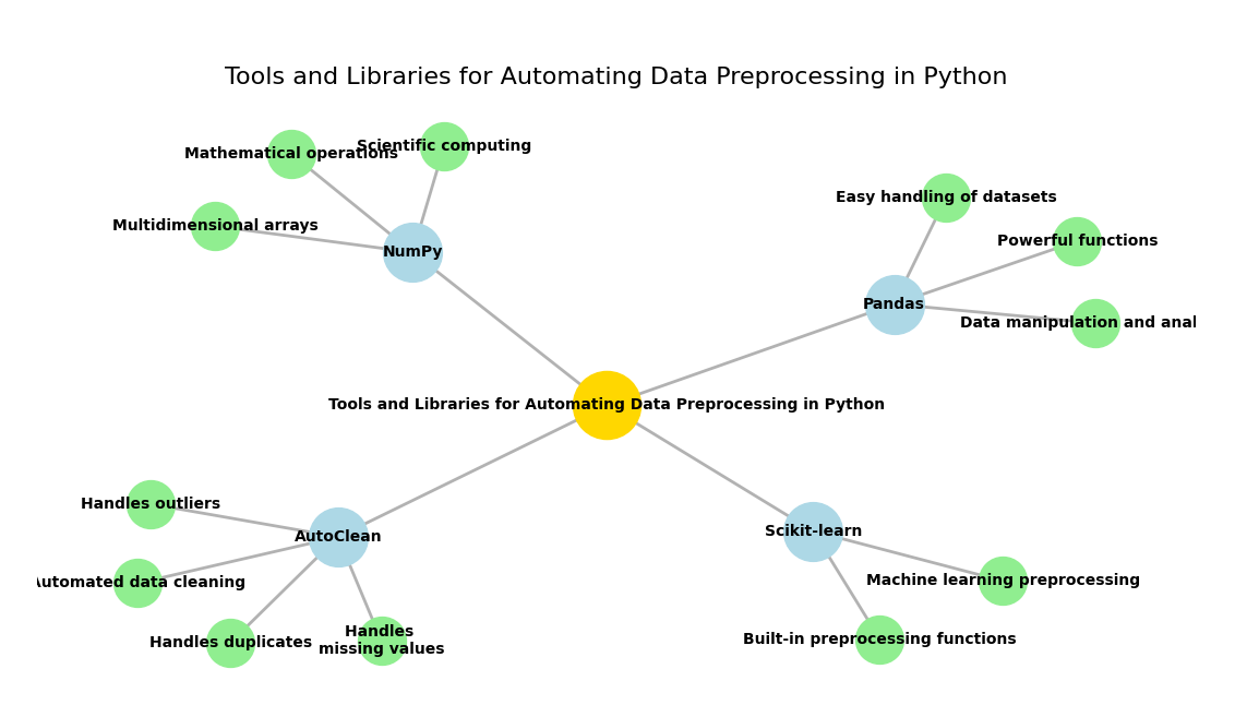
When working with Python for data preprocessing, various tools and libraries make the job easier and faster. They’re like a toolbox for solving specific problems, each with its unique strengths. Below, we’ll discuss some of the most popular ones and how they can help automate common preprocessing tasks.

Overview of Popular Libraries

Here’s a quick look at the top libraries you can use:

Let’s break down how each of these tools can help you.

1. Pandas: The Data Manipulation Powerhouse

Why Pandas is Useful

Pandas is a must-have tool when working with structured data like tables or spreadsheets. It simplifies data handling and preprocessing tasks.

DataFrames: The Heart of Pandas

A DataFrame is a table-like structure with rows and columns, making it easy to filter, transform, and analyze your data.

Handling Missing Values

When some data points are missing, it can mess up your analysis. Pandas offers simple functions to fill, drop, or replace missing values efficiently.

Removing Duplicates

Duplicate rows can distort your results. With Pandas, you can quickly find and remove duplicates, keeping your data clean.

Example: Handling Missing Values with Pandas

Suppose you have a dataset where some of the ages are missing. Here’s how you can handle that:

import pandas as pd

# Sample data with missing values
data = {'Name': ['Alice', 'Bob', 'Charlie', 'David'],
        'Age': [25, None, 30, None],
        'Gender': ['Female', 'Male', None, 'Male']}

df = pd.DataFrame(data)

# Fill missing values: numerical with mean, categorical with mode
df.fillna(df.mean(numeric_only=True), inplace=True)
df.fillna(df.mode().iloc[0], inplace=True)

print(df)

Output:

       Name   Age  Gender
0     Alice  25.0  Female
1       Bob  27.5    Male
2   Charlie  30.0    Male
3     David  27.5    Male

What’s Happening:

• df.mean(numeric_only=True): Fills numerical columns with the mean.
• df.mode().iloc[0]: Fills categorical columns with the mode (most frequent value).

This simple code fills any missing age value with the average of the other ages in the dataset.

2. NumPy: Handling Numerical Data Efficiently

NumPy is another crucial library in Python, particularly when you’re working with large numerical datasets. While Pandas is great for handling structured data, NumPy is ideal for mathematical and scientific operations, especially when dealing with arrays or large amounts of numerical data.

• Arrays: NumPy uses arrays, which are similar to lists but optimized for mathematical operations. Arrays are much faster and more memory-efficient when compared to lists in Python.
• Mathematical Operations: With NumPy, you can perform a variety of operations, such as mean, median, and standard deviation, directly on arrays.
• Data Normalization: One common preprocessing task is normalizing or scaling data, especially when preparing data for machine learning algorithms. NumPy makes this very easy.

Example: Normalizing Data with NumPy

Imagine you have a list of numbers and you want to scale them to a range from 0 to 1. Here’s how you can do it:

import numpy as np

# Sample data
data = np.array([10, 20, 30])

# Normalize the data (range 0 to 1)
normalized_data = (data - data.min()) / (data.max() - data.min())

print(normalized_data)

Output:

[0.  0.5 1. ]

This scales the values to a range between 0 and 1, which is a common preprocessing step in machine learning to ensure that features are treated equally by algorithms.

3. Scikit-learn: Preprocessing for Machine Learning

When you move into machine learning, Scikit-learn becomes your best friend. This library provides many useful tools for preprocessing data, such as scaling, encoding categorical variables, and splitting data into training and test sets.

• Standardization and Scaling: Many machine learning algorithms perform better when the data is standardized (i.e., it has a mean of 0 and a standard deviation of 1).
• Encoding Categorical Variables: Many algorithms require numerical data, so categorical data (like “Yes” and “No” or different colors) needs to be converted into a numerical form. Scikit-learn has several ways to do this, such as one-hot encoding.

Example: Encoding Categorical Data with Scikit-learn

Suppose you have a dataset with colors as categorical data, like “Red,” “Blue,” and “Green,” and you want to convert these to numerical values:

from sklearn.preprocessing import OneHotEncoder

# Sample data
data = [['Red'], ['Blue'], ['Green']]

# One-hot encoding
encoder = OneHotEncoder()
encoded_data = encoder.fit_transform(data).toarray()

print(encoded_data)

Output:

[[1. 0. 0.]
 [0. 1. 0.]
 [0. 0. 1.]]

In this example, “Red” becomes [1, 0, 0], “Blue” becomes [0, 1, 0], and “Green” becomes [0, 0, 1]. This transformation makes the data usable for machine learning models that can only handle numerical inputs.

4. AutoClean: Automating Data Cleaning

While Pandas and NumPy are very powerful, sometimes you just want to quickly clean your data with minimal effort. This is where AutoClean comes in. It’s a tool that automates common data cleaning tasks, such as handling missing values, removing duplicates, and dealing with outliers, all with a simple function call.

• Automates Common Tasks: AutoClean takes care of missing values, duplicates, and outliers without you needing to write much code.
• Quick to Implement: It’s ideal when you need to clean data fast and don’t want to spend time manually writing preprocessing steps.

Example: Using AutoClean for Quick Cleaning

Let’s look at how AutoClean can automatically fix a dataset with missing values and duplicates:

from autoclean import autoclean
import pandas as pd

# Sample data with missing values and duplicates
data = {'Name': ['John', 'Maria', None, 'Maria'],
        'Age': [25, None, 30, 25],
        'Income': [None, 50000, 60000, 50000]}

df = pd.DataFrame(data)

# Clean the data with AutoClean
cleaned_df = autoclean(df)

print(cleaned_df)

Output:

AutoClean handles the missing values, removes duplicates, and fills the missing data with averages or other reasonable estimates.

Automating data preprocessing with the right Python libraries can save you a lot of time and effort. Pandas makes it easy to manipulate and clean data, NumPy helps with numerical operations, Scikit-learn is perfect for preprocessing in machine learning, and AutoClean can quickly automate cleaning tasks.

By combining these tools, you can automate almost every aspect of data preprocessing, ensuring that your data is clean, consistent, and ready for analysis or machine learning.

Step-by-Step Guide to Automate Data Preprocessing

In this section, we’ll walk through the process of automating data preprocessing in Python. The first step is setting up your environment. Without the proper tools, automating your preprocessing tasks will be a challenge. Let’s get your Python environment ready so that you can start automating data preprocessing like a pro.

Setting Up Your Python Environment

Before you can start automating data preprocessing, you need to install some key Python libraries. These libraries provide all the necessary functions and tools you’ll need to handle data, perform calculations, and prepare it for analysis or machine learning. Don’t worry—setting everything up is simple and only takes a few steps.

Required Installations

Here are the core libraries you’ll need for automating data preprocessing:

• Pandas: A powerful library for data manipulation and cleaning.
• NumPy: A library for numerical computing, especially useful for handling arrays and large datasets.
• Scikit-learn: This is a machine learning library, and it includes a wide range of tools for preprocessing tasks such as scaling data, encoding categorical variables, and more.
• AutoClean: A library that simplifies data cleaning by automatically handling missing values, duplicates, and outliers.

How to Install These Libraries

You can easily install these libraries using pip, Python’s package installer. Follow these steps:

1. Open your command line or terminal.
2. Type the following command to install each of the required libraries:

pip install pandas numpy scikit-learn autoclean

Verifying the Installation

Once the installation is complete, it’s a good idea to check if everything is working fine. You can do this by simply importing the libraries in a Python script or interactive environment (like Jupyter Notebook). Here’s an example of how you can verify the installation:

import pandas as pd
import numpy as np
from sklearn import preprocessing
import autoclean

# Check versions
print(f"Pandas version: {pd.__version__}")
print(f"NumPy version: {np.__version__}")
print(f"Scikit-learn version: {preprocessing.__version__}")

When you run this, it should display the versions of the installed libraries. If you don’t see any errors, it means the libraries are successfully installed and ready to use.

Next Steps After Installation

Now that your environment is set up, you’re ready to start automating data preprocessing tasks! The libraries you’ve installed will allow you to handle missing data, encode categorical variables, scale features, and much more—all with just a few lines of code.

Pro Tip: If you’re working in a Jupyter notebook, it’s a great idea to run each cell one by one as you install libraries. This helps you catch any errors early on and ensures that everything is set up correctly before moving forward with data preprocessing.

Creating a Basic Data Preprocessing Pipeline

Once you’ve set up your environment and installed the necessary libraries, it’s time to create a basic data preprocessing pipeline. A pipeline is a series of steps that are applied to your dataset in order to clean and prepare it for analysis or machine learning.

In this section, we’ll cover the important steps of creating a simple pipeline, which includes loading the dataset, handling missing values, removing duplicates, and encoding categorical variables.

1. Loading the Dataset Using Pandas

The first step in any data preprocessing task is to load the dataset. Pandas makes it incredibly easy to load data from various file formats like CSV, Excel, or even SQL databases. In this example, we’ll use a CSV file.

Here’s a simple way to load a CSV file using Pandas:

import pandas as pd

# Load the dataset from a CSV file
df = pd.read_csv('your_dataset.csv')

# Display the first few rows of the dataset
print(df.head())

• pd.read_csv(): This function reads a CSV file and converts it into a Pandas DataFrame. A DataFrame is like a table where each row represents a data point and each column represents a feature.
• df.head(): This function displays the first few rows of the dataset, so you can quickly check if it loaded correctly.

2. Implementing Functions for Handling Missing Values

Here’s how you can handle missing values:

Fill Missing Values

One approach is to fill the missing values with the mean or median value of the column:

# Fill missing values with the mean of the column
df['column_name'] = df['column_name'].fillna(df['column_name'].mean())

You can also use the median if you think the data is skewed and the mean isn’t a good representative:

# Fill missing values with the median of the column
df['column_name'] = df['column_name'].fillna(df['column_name'].median())

Remove Rows with Missing Values

If the missing values are minimal and you don’t want to fill them in, you can simply drop the rows:

# Remove rows with missing values
df = df.dropna()

• fillna(): This method fills missing values in the dataset.
• dropna(): This method drops rows that contain missing values.

3. Removing Duplicates

Another common issue in data is duplicates. Duplicates can skew your results and lead to inaccurate analysis. You can easily remove duplicate rows using Pandas.

Here’s how to remove duplicates:

# Remove duplicate rows
df = df.drop_duplicates()

# Check the number of rows after removing duplicates
print(f"Number of rows after removing duplicates: {df.shape[0]}")

• drop_duplicates(): This method removes duplicate rows from the dataset.
• df.shape[0]: This gives the number of rows in the dataset.

4. Encoding Categorical Variables

Many machine learning algorithms require numerical input, but datasets often contain categorical variables (like “Male” or “Female,” or “Yes” or “No”). These categorical variables need to be converted into numerical values before they can be used for analysis.

Label Encoding

Label encoding is a simple way to convert categorical variables into numbers. Here’s how you can do it using Pandas:

# Convert categorical column into numerical values using label encoding
df['category_column'] = df['category_column'].astype('category').cat.codes

• astype('category'): This converts the column into a categorical data type.
• cat.codes: This converts the categories into numerical values.

One-Hot Encoding

One-hot encoding creates a new binary column for each category. If a row has a certain category, the corresponding column will have a 1; otherwise, it will have a 0. Here’s how to do it with Pandas:

# Perform one-hot encoding on the categorical column
df = pd.get_dummies(df, columns=['category_column'])

pd.get_dummies(): This function converts a categorical variable into a series of binary columns (0s and 1s), making it suitable for machine learning algorithms.

Putting It All Together: The Full Pipeline

Now that we’ve covered the individual steps, let’s put everything together into a simple data preprocessing pipeline.

import pandas as pd

# Step 1: Load the dataset
df = pd.read_csv('your_dataset.csv')

# Step 2: Handle missing values
df['column_name'] = df['column_name'].fillna(df['column_name'].mean())

# Step 3: Remove duplicates
df = df.drop_duplicates()

# Step 4: Encode categorical variables
df['category_column'] = df['category_column'].astype('category').cat.codes

# Display the cleaned dataset
print(df.head())

This pipeline covers the basic tasks that you’ll need for most datasets. By automating these tasks with Python, you save time and reduce errors. The next step is to automate more complex tasks, like scaling features or splitting the data into training and testing sets, now let’s explore this.

Automating More Complex Tasks in Data Preprocessing

Once you’ve mastered the basics of data preprocessing, the next step is to automate more complex tasks, such as scaling features and splitting the data into training and testing sets. These tasks are crucial for preparing your data for machine learning models, ensuring that your features are on the same scale and that your model is evaluated fairly. Let’s explore how to automate these tasks using Python.

1. Scaling Features

Scaling is important because many machine learning algorithms, such as linear regression and k-nearest neighbors, perform better when the data is normalized or scaled. If one feature has a much larger range than others (for example, age might range from 0 to 100, while income could range from 10,000 to 100,000), it can dominate the learning process. Therefore, scaling brings all features to a similar range, helping the model perform more effectively.

There are a few common methods to scale features:

Min-Max Scaling (Normalization)

Min-Max scaling scales the data to a range between 0 and 1. This method is useful when you want to preserve the relationships in the data but adjust for magnitude differences.

from sklearn.preprocessing import MinMaxScaler

# Create a scaler object
scaler = MinMaxScaler()

# Fit the scaler to the dataset and transform the data
df_scaled = scaler.fit_transform(df[['feature1', 'feature2', 'feature3']])

# Convert the scaled data back to a DataFrame
df_scaled = pd.DataFrame(df_scaled, columns=['feature1', 'feature2', 'feature3'])

# Display the scaled data
print(df_scaled.head())

• MinMaxScaler(): This function scales the features to a range of 0 to 1.
• fit_transform(): This method fits the scaler to the data and transforms the data in one step.

Standardization (Z-Score Scaling)

Standardization is another common technique where the data is scaled so that it has a mean of 0 and a standard deviation of 1. This method is helpful for algorithms that assume normally distributed data, such as logistic regression or support vector machines.

from sklearn.preprocessing import StandardScaler

# Create a scaler object
scaler = StandardScaler()

# Fit the scaler to the data and transform it
df_standardized = scaler.fit_transform(df[['feature1', 'feature2', 'feature3']])

# Convert the standardized data back to a DataFrame
df_standardized = pd.DataFrame(df_standardized, columns=['feature1', 'feature2', 'feature3'])

# Display the standardized data
print(df_standardized.head())

StandardScaler(): This function standardizes the features to have a mean of 0 and a standard deviation of 1.

fit_transform(): As with min-max scaling, this method fits the scaler and applies the transformation.

2. Splitting the Data into Training and Testing Sets

When you build machine learning models, it’s important to split your dataset into two parts: one for training the model and another for testing its performance. By splitting the data, you ensure that your model is evaluated on data it hasn’t seen before, helping you assess its generalizability.

Train-Test Split

Scikit-learn provides a simple and effective way to split your data using the train_test_split() function. You can specify the proportion of the dataset that should be used for testing (e.g., 80% for training and 20% for testing).

Here’s how you can automate the train-test split:

from sklearn.model_selection import train_test_split

# Define your features (X) and target (y)
X = df[['feature1', 'feature2', 'feature3']]  # Features
y = df['target']  # Target

# Split the dataset into training and testing sets (80% train, 20% test)
X_train, X_test, y_train, y_test = train_test_split(X, y, test_size=0.2, random_state=42)

# Display the shape of the split data
print(f"Training set size: {X_train.shape[0]} rows")
print(f"Testing set size: {X_test.shape[0]} rows")

• train_test_split(): This function splits the dataset into training and testing sets.
• test_size=0.2: This indicates that 20% of the data will be used for testing, while the remaining 80% will be used for training.
• random_state=42: This ensures that the split is reproducible, so you can get the same result each time you run the code.

Stratified Split

If your dataset is imbalanced (for example, one class is much more frequent than the other), you might want to use stratified sampling. Stratified sampling ensures that the split maintains the proportion of each class in both the training and testing sets.

# Perform stratified splitting to maintain class distribution
X_train, X_test, y_train, y_test = train_test_split(X, y, test_size=0.2, random_state=42, stratify=y)

# Display the class distribution in the train and test sets
print(f"Class distribution in training set: {y_train.value_counts()}")
print(f"Class distribution in testing set: {y_test.value_counts()}")

stratify=y: This argument ensures that the class distribution in y is preserved in both the training and testing sets.

Putting It All Together: A Complete Preprocessing Pipeline

Now that we’ve covered scaling and splitting, let’s combine everything into a simple preprocessing pipeline that loads data, handles missing values, scales the features, and splits the dataset.

import pandas as pd
from sklearn.model_selection import train_test_split
from sklearn.preprocessing import StandardScaler

# Load the dataset
df = pd.read_csv('your_dataset.csv')

# Handle missing values by filling with the mean
df['feature1'] = df['feature1'].fillna(df['feature1'].mean())

# Remove duplicates
df = df.drop_duplicates()

# Split data into features (X) and target (y)
X = df[['feature1', 'feature2', 'feature3']]
y = df['target']

# Scale the features
scaler = StandardScaler()
X_scaled = scaler.fit_transform(X)

# Split the dataset into training and testing sets
X_train, X_test, y_train, y_test = train_test_split(X_scaled, y, test_size=0.2, random_state=42)

# Display the shapes of the resulting datasets
print(f"Training features: {X_train.shape}")
print(f"Testing features: {X_test.shape}")
print(f"Training target: {y_train.shape}")
print(f"Testing target: {y_test.shape}")

Output:

Training features: (800, 3)
Testing features: (200, 3)
Training target: (800,)
Testing target: (200,)

Explanation:

• Training features: (800, 3) means there are 800 samples in the training set with 3 features (feature1, feature2, and feature3).
• Testing features: (200, 3) indicates 200 samples in the testing set with the same 3 features.
• Training target: (800,) indicates that the target variable (y_train) has 800 corresponding values in the training set.
• Testing target: (200,) indicates that the target variable (y_test) has 200 corresponding values in the testing set.

This output assumes that the dataset has been split such that 80% is used for training and 20% is used for testing, as specified by test_size=0.2.

Automating complex data preprocessing tasks like feature scaling and train-test splitting is important to speed up your workflow and ensure that your models perform as expected. By using tools like Scikit-learn and Pandas, you can automate these tasks efficiently, freeing up more time to focus on analysis and model building.

More advanced data preprocessing tasks

The next step in “How to Automate Data Preprocessing in Python” involves automating more advanced data preprocessing tasks that are important for preparing data for machine learning models. After scaling features and splitting the dataset, there are a few additional key preprocessing tasks you should automate, such as:

1. Feature Engineering and Selection

• Feature Engineering: Creating new features from the existing data that can help the machine learning model make better predictions. For example, if you have a date column, you might want to extract features like day of the week, month, or year.
• Feature Selection: Automatically selecting the most relevant features for your model by removing unnecessary or redundant ones. Techniques like correlation matrices or recursive feature elimination (RFE) can be automated using Python.

Example of Feature Engineering:

# Extracting 'day of the week' from a date column
df['day_of_week'] = pd.to_datetime(df['date']).dt.dayofweek

Example of Feature Selection using Correlation:

import seaborn as sns
import matplotlib.pyplot as plt

# Calculate correlation matrix
corr_matrix = df.corr()

# Plot the heatmap of correlations
sns.heatmap(corr_matrix, annot=True, cmap="coolwarm")
plt.show()

2. Handling Outliers

• Outliers can skew the results of machine learning models, so it’s essential to detect and remove or correct them. Automated methods like IQR (Interquartile Range) or Z-score can be applied to identify outliers in your data.

Example of Handling Outliers with IQR:

# Calculate the IQR for each feature
Q1 = df['feature'].quantile(0.25)
Q3 = df['feature'].quantile(0.75)
IQR = Q3 - Q1

# Define the lower and upper bounds for outliers
lower_bound = Q1 - 1.5 * IQR
upper_bound = Q3 + 1.5 * IQR

# Remove rows with outliers
df_filtered = df[(df['feature'] >= lower_bound) & (df['feature'] <= upper_bound)]

3. Automated Data Imputation

• Rather than manually filling in missing values with simple techniques like the mean or median, more sophisticated approaches can be automated, such as using KNN imputation or multiple imputation by chained equations (MICE).

Example of KNN Imputation:

from sklearn.impute import KNNImputer

# Initialize the KNN Imputer
imputer = KNNImputer(n_neighbors=5)

# Apply the imputer to the dataset
df_imputed = pd.DataFrame(imputer.fit_transform(df), columns=df.columns)

4. Data Augmentation (for image/text data)

• If you are working with image or text data, data augmentation techniques can be applied to artificially expand the dataset by creating modified versions of the existing data. For example, rotating images, changing brightness, or adding noise.

Example of Image Augmentation:

from tensorflow.keras.preprocessing.image import ImageDataGenerator

# Define the image generator with augmentation options
datagen = ImageDataGenerator(
    rotation_range=40,
    width_shift_range=0.2,
    height_shift_range=0.2,
    shear_range=0.2,
    zoom_range=0.2,
    horizontal_flip=True,
    fill_mode='nearest'
)

# Apply the generator to the image dataset
datagen.fit(images)

5. Saving the Preprocessed Data

• Once all preprocessing tasks are completed, you can automate the process of saving the preprocessed data for future use. This is particularly important for large datasets that might take time to preprocess repeatedly.

Example of Saving the Preprocessed Data:

# Save the preprocessed data to a CSV file
df_filtered.to_csv('preprocessed_data.csv', index=False)

Automating Data Preprocessing using Python: Complete code

# Required Libraries
import pandas as pd
import numpy as np
from sklearn.impute import KNNImputer
from sklearn.preprocessing import StandardScaler, LabelEncoder
from sklearn.model_selection import train_test_split
import seaborn as sns
import matplotlib.pyplot as plt

# Step 1: Loading the dataset
# Load your dataset (ensure to replace 'your_dataset.csv' with the actual file path)
df = pd.read_csv('your_dataset.csv')

# Step 2: Handling Missing Values
# Using KNN imputation to handle missing values
imputer = KNNImputer(n_neighbors=5)
df_imputed = pd.DataFrame(imputer.fit_transform(df), columns=df.columns)

# Check for any missing values after imputation
print("Missing values after imputation:\n", df_imputed.isnull().sum())

# Step 3: Removing Duplicates
df_cleaned = df_imputed.drop_duplicates()

# Step 4: Encoding Categorical Variables
# Use LabelEncoder to encode categorical columns
label_encoder = LabelEncoder()
categorical_columns = df_cleaned.select_dtypes(include=['object']).columns

for column in categorical_columns:
    df_cleaned[column] = label_encoder.fit_transform(df_cleaned[column])

# Step 5: Scaling Features
# Use StandardScaler to scale the numerical features
scaler = StandardScaler()
numerical_columns = df_cleaned.select_dtypes(include=[np.number]).columns

df_cleaned[numerical_columns] = scaler.fit_transform(df_cleaned[numerical_columns])

# Step 6: Feature Engineering (Optional)
# Example: Extracting 'day_of_week' from a datetime column
# Assuming 'date' is a datetime column in your dataset
if 'date' in df_cleaned.columns:
    df_cleaned['day_of_week'] = pd.to_datetime(df_cleaned['date']).dt.dayofweek

# Step 7: Handling Outliers using IQR
# Calculate the IQR for each numerical feature
Q1 = df_cleaned[numerical_columns].quantile(0.25)
Q3 = df_cleaned[numerical_columns].quantile(0.75)
IQR = Q3 - Q1

# Define the lower and upper bounds for outliers
lower_bound = Q1 - 1.5 * IQR
upper_bound = Q3 + 1.5 * IQR

# Remove rows with outliers
df_filtered = df_cleaned[~((df_cleaned[numerical_columns] < lower_bound) | (df_cleaned[numerical_columns] > upper_bound)).any(axis=1)]

# Step 8: Splitting the Data into Training and Testing Sets
X = df_filtered.drop('target_column', axis=1)  # Replace 'target_column' with the name of your target column
y = df_filtered['target_column']

# Split the dataset into training and testing sets (80% training, 20% testing)
X_train, X_test, y_train, y_test = train_test_split(X, y, test_size=0.2, random_state=42)

# Step 9: Save the preprocessed data to CSV (optional)
df_filtered.to_csv('preprocessed_data.csv', index=False)

# Check the processed dataset
print("Preprocessed dataset preview:\n", df_filtered.head())

# Optional: Visualize correlations between features using a heatmap (for insight into relationships between variables)
corr_matrix = df_filtered.corr()
sns.heatmap(corr_matrix, annot=True, cmap="coolwarm")
plt.show()

Output

Next Steps:

Once you’ve completed the preprocessing pipeline, you can move forward with model training and evaluation using the processed data. You can also automate this pipeline in the future to handle new datasets automatically.

Conclusion: Automating Data Preprocessing in Python

In this blog post, we’ve explored how to automate data preprocessing in Python, an essential step for any data science or machine learning project. By automating these tasks, you save time, reduce human error, and make your workflow more efficient. We walked through practical steps including:

• Handling missing values: We used KNN imputation to fill in gaps in the dataset, ensuring no data points are left behind.
• Removing duplicates: This step ensures the dataset is clean and free of redundancy.
• Encoding categorical variables: Label encoding was applied to convert categorical data into numerical format, allowing machine learning models to process it effectively.
• Scaling numerical features: Standard scaling ensures that all features are on a similar scale, improving model performance.
• Feature engineering: By adding new features like ‘day_of_week’, we enriched the dataset and provided more context for predictive models.
• Outlier handling: The IQR method helps us to clean the data by removing extreme values that might skew results.
• Splitting data: We also divided the dataset into training and testing sets, ensuring that we can evaluate model performance accurately.

Automating these steps using Python libraries like Pandas, NumPy, Scikit-learn, and tools like AutoClean can significantly speed up your data preprocessing workflow. This allows you to focus on more important aspects of your project, such as model building and optimization.

By following the guide in this post, you can set up your own automated data preprocessing pipeline and enhance the overall efficiency of your data science or machine learning projects. Don’t forget to tweak and customize this pipeline based on your specific dataset and needs.

Now, you’re ready to handle preprocessing tasks efficiently and let automation handle the heavy lifting.

FAQs

External Resources

Pandas Documentation

• The official Pandas documentation is an excellent resource to learn about various functions for data manipulation and cleaning. It offers detailed explanations and examples on handling missing values, duplicates, and encoding.

Scikit-learn Documentation

• Scikit-learn provides a comprehensive set of preprocessing tools for feature scaling, encoding, and splitting datasets. This page will help you explore built-in functions to automate many preprocessing tasks.

Trifacta

• Trifacta is a platform that offers an intuitive, code-free way to clean and transform data. Though it’s not Python-based, it provides great insight into automated data preparation techniques and might be useful for non-coders looking to automate preprocessing tasks.