

Top 8 Hidden Python Libraries for Machine Learning That Will Supercharge Your Models
Introduction
Python Libraries for Machine Learning: Python is the top choice for machine learning because it has so many useful libraries. You’ve probably heard of TensorFlow, PyTorch, and Scikit-learn—they’re the most popular ones.
But did you know there are lesser-known libraries that can make machine learning even faster, easier, and more powerful? These hidden tools can save you time, improve your models, and simplify complex tasks.
In this post, we’ll share top 8 hidden Python libraries that can boost your machine learning projects and help you work smarter. Let’s get started!
JAX – Faster NumPy with Auto-Differentiation
When working on machine learning projects, speed is the most important one. Large datasets and complex models can slow down your computations. Which makes your training and testing take longer. That’s why we use JAX. It’s one of the best Python libraries for machine learning. If you want for faster calculations and built-in differentiation then JAX is the best choice. Now let’s see what is JAX. How we can use it in our machine learning projects.
What is JAX?
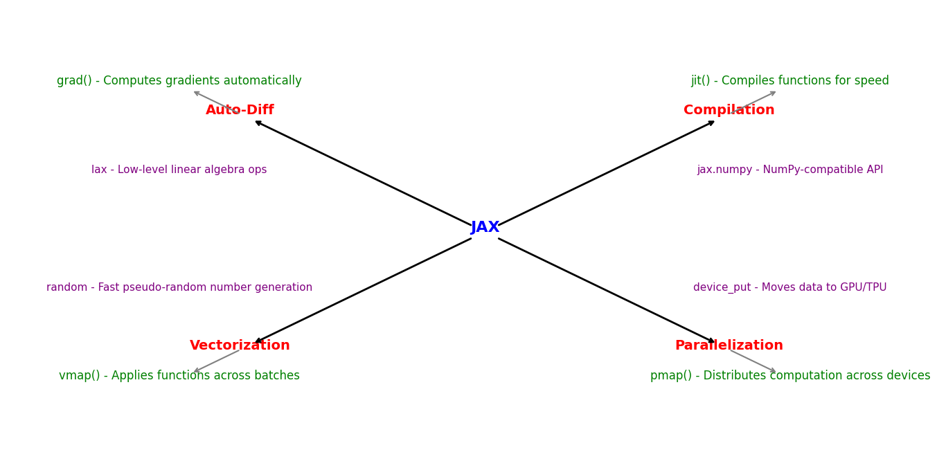
JAX is a library developed by Google that works just like NumPy, but much faster. It can automatically compute gradients (which is important for training machine learning models) and run code efficiently on CPUs, GPUs, and TPUs.
Why is JAX Better than NumPy?
- Speed Boost – JAX uses XLA (Accelerated Linear Algebra) to optimize code execution, making it much faster than traditional NumPy.
- Auto-Differentiation – It can automatically compute derivatives and gradients, which is useful for machine learning and deep learning.
- GPU & TPU Support – Unlike NumPy, which mainly runs on CPUs, JAX can take full advantage of GPUs and TPUs for faster model training.
- Just-in-Time (JIT) Compilation – JAX can compile functions to run them even faster, reducing computation time.
How Does JAX Work? (With Code Example)
Let’s see how JAX helps with auto-differentiation. We use Auto-differentiation to update model weights during training.
import jax.numpy as jnp
from jax import grad

# Define a simple mathematical function
def func(x):
    return x**2 + 3*x + 2

# Compute the gradient (derivative) of the function
grad_func = grad(func)

# Find the gradient at x = 2
print(grad_func(2.0))  # Output: 7.0
Breaking Down the Code:
- We import
jax.numpy(which works just like regular NumPy). - We define a function
func(x) = x² + 3x + 2. - The
grad()function automatically finds the derivative of our function. - When we call
grad_func(2.0), it calculates the slope at x = 2, which is7.
This is extremely useful in machine learning because models need to compute gradients during training to adjust weights. JAX does this efficiently and quickly.
Should You Use JAX?
If you’re working with deep learning, large datasets, or scientific computing, JAX can significantly speed up your workflow. Since it works similarly to NumPy, you don’t need to completely rewrite your code—just make a few changes to take advantage of its power.
Now let’s see how we can replace numpy without rewrite our complete code.
How to Rewrite NumPy Code for JAX
If you’re already using NumPy in your machine learning projects, switching to JAX is easy. JAX provides a NumPy-like interface, so you only need to make a few changes. Let’s go step by step.
Import JAX Instead of NumPy
Before (NumPy Code):
import numpy as np

x = np.array([1.0, 2.0, 3.0])
print(np.sin(x))  # Compute sine
After (JAX Code):
import jax.numpy as jnp

x = jnp.array([1.0, 2.0, 3.0])
print(jnp.sin(x))  # Compute sine
Only the import changes from numpy to jax.numpy, but everything else stays the same.
Use jax.numpy Instead of numpy for Arrays and Operations
JAX functions behave just like NumPy, so you can rewrite most of your NumPy code by simply replacing np with jnp.
Before (NumPy Code):
import numpy as np

A = np.random.rand(3, 3)  # Create a 3x3 random matrix
B = np.linalg.inv(A)  # Compute inverse
print(B)
After (JAX Code):
import jax.numpy as jnp

A = jnp.random.rand(3, 3)  # Create a 3x3 random matrix
B = jnp.linalg.inv(A)  # Compute inverse
print(B)
The code remains almost identical, except we use jnp instead of np.
Add jit for Faster Computation
JAX has a powerful Just-in-Time (JIT) compiler that makes functions run much faster. You can speed up your NumPy-like operations using jax.jit().
Before (Regular NumPy Code):
import numpy as np

def compute(x):
    return np.sin(x) + np.cos(x)

x = np.linspace(0, 10, 1000)
y = compute(x)
After (Optimized JAX Code with JIT):
import jax.numpy as jnp
from jax import jit

@jit  # Compile the function for better performance
def compute(x):
    return jnp.sin(x) + jnp.cos(x)

x = jnp.linspace(0, 10, 1000)
y = compute(x)  # Runs much faster with JIT!
The jit decorator compiles the function, making it run faster on CPUs, GPUs, or TPUs.
Use grad() for Automatic Differentiation
JAX can automatically compute gradients, which is a game-changer for machine learning.
Before (Manual Derivative in NumPy):
import numpy as np

def func(x):
    return x**2 + 3*x + 2

def manual_derivative(x):
    return 2*x + 3  # Manually computed derivative

print(manual_derivative(2.0))  # Output: 7.0
After (Auto-Differentiation with JAX):
import jax.numpy as jnp
from jax import grad

def func(x):
    return x**2 + 3*x + 2

grad_func = grad(func)  # JAX automatically computes the derivative
print(grad_func(2.0))  # Output: 7.0
JAX eliminates the need to manually calculate gradients—just use grad()!
Move Computations to GPU/TPU Easily
With JAX, you don’t need to manually set up a GPU. It automatically runs operations on a GPU (if available). But you can explicitly move data to a GPU or TPU if needed.
import jax.numpy as jnp
from jax import device_put

x = jnp.array([1.0, 2.0, 3.0])

# Move data to GPU
x_gpu = device_put(x)

print(x_gpu.device())  # Should print something like "gpu:0" if GPU is available
No need for torch.cuda() or manual device handling—JAX does it for you!
JAX is one of the most underrated Python libraries for machine learning, and if you’re looking to optimize performance, it’s definitely worth exploring!
Flax – Lightweight Neural Networks with JAX
When working with Python libraries for machine learning, you’re probably already familiar with TensorFlow and PyTorch for building neural networks. But if you want faster training, GPU acceleration, and better performance, Flax is an excellent alternative. It’s a lightweight deep learning library built on top of JAX, making it easy to build and train neural networks efficiently.
What is Flax?
Flax is a neural network library built for JAX. It helps you create and train deep learning models efficiently.
Key Features:
- Flexible and modular neural network layers
- Automatic differentiation powered by JAX
- GPU/TPU acceleration for faster training
- Seamless integration with JAX’s Just-in-Time (JIT) compilation
Unlike TensorFlow and PyTorch, Flax is lightweight and highly customizable, making it a great choice for research and high-performance machine learning models.
Why Use Flax?
- Faster Model Training – Since Flax runs on JAX, it takes full advantage of JIT compilation, making neural networks train much faster.
- GPU & TPU Support – Unlike standard NumPy-based frameworks, Flax runs efficiently on CPUs, GPUs, and TPUs without extra setup.
- Clear and Modular Design – It’s designed to be easy to use and extend, making it great for both beginners and advanced researchers.
- Works Seamlessly with JAX – If you’re already using JAX, Flax integrates perfectly without additional dependencies.
How to Build a Neural Network with Flax
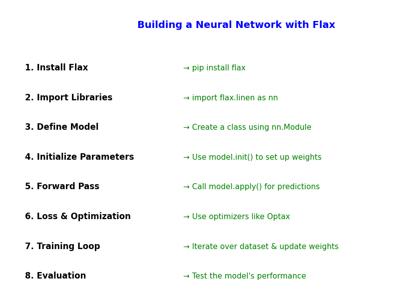
Let’s see how to create a simple neural network using Flax and JAX.
Step 1: Install Flax
First, install the required libraries:
pip install flax jax jaxlib optax
Step 2: Import Required Libraries
import jax.numpy as jnp
import jax.random as random
import flax.linen as nn
from jax import grad, jit
flax.linen– Flax’s module for defining neural networksjax.numpy– JAX’s version of NumPy for faster calculationsjax.random– Used for initializing model parameters
Step 3: Define a Simple Neural Network
Flax makes it easy to define neural networks using nn.Module:
class SimpleNN(nn.Module):
    @nn.compact  # Marks layers inside the model
    def __call__(self, x):
        x = nn.Dense(features=128)(x)  # Hidden layer with 128 neurons
        x = nn.relu(x)  # Activation function
        x = nn.Dense(features=10)(x)   # Output layer with 10 neurons
        return x
What’s happening here?
- The model takes input
x. - It has a dense (fully connected) layer with 128 neurons.
- We use ReLU activation to introduce non-linearity.
- The final output layer has 10 neurons (for classification tasks like MNIST).
Step 4: Initialize and Run the Model
# Create a random input tensor
key = random.PRNGKey(0)  # Random seed
x = jnp.ones((1, 20))  # Example input with 20 features

# Initialize model
model = SimpleNN()
params = model.init(key, x)  # Initialize weights
output = model.apply(params, x)  # Run forward pass

print(output)
Breaking it down:
- We initialize random weights using
model.init(). model.apply()runs a forward pass, computing the model’s predictions.- Since JAX doesn’t store state like PyTorch, we always pass
paramsexplicitly.
Step 5: Training the Model with Flax and Optax
Flax doesn’t come with an optimizer, but Optax (another JAX library) makes it easy to train neural networks.
import optax

# Define loss function (Mean Squared Error)
def loss_fn(params, x, y):
    predictions = model.apply(params, x)
    return jnp.mean((predictions - y) ** 2)  # MSE Loss

# Compute gradient automatically using JAX
grad_fn = jax.grad(loss_fn)

# Define optimizer (SGD)
optimizer = optax.sgd(learning_rate=0.01)
opt_state = optimizer.init(params)

# Apply gradients
grads = grad_fn(params, x, jnp.ones((1, 10)))  # Dummy target
updates, opt_state = optimizer.update(grads, opt_state)
params = optax.apply_updates(params, updates)
Key takeaways:
loss_fn()computes the loss.jax.grad(loss_fn)automatically finds gradients.- Optax provides optimizers like SGD, Adam, and RMSprop.
- We update the model’s parameters using
optax.apply_updates().
Flax vs PyTorch vs TensorFlow
| Feature | Flax (JAX) | PyTorch | TensorFlow |
|---|---|---|---|
| Speed | 🚀 Fastest (JIT + XLA) | ✅ Fast | ❌ Slower |
| GPU/TPU Support | ✅ Built-in | ✅ Yes | ✅ Yes |
| Automatic Differentiation | ✅ Yes (grad) | ✅ Yes (autograd) | ✅ Yes (TF.GradientTape) |
| Flexibility | ✅ Highly modular | ✅ Good | ❌ Less flexible |
| Ecosystem | ⚡ Research-focused | 🌍 Industry & research | 🏢 Enterprise use |
Flax is the best choice for speed and flexibility, especially for research and high-performance ML models!
If you’re looking for a lightweight and powerful neural network library, Flax is an amazing alternative to PyTorch and TensorFlow. Since it’s built on JAX, it provides faster training, automatic differentiation, and seamless GPU acceleration.
LightGBM – The Fastest Gradient Boosting Library
When working with Python libraries for machine learning, LightGBM (Light Gradient Boosting Machine) is an important tool for training high-performance models quickly. If you’ve used XGBoost, you’ll love LightGBM because it’s faster, uses less memory, and handles large datasets efficiently.
What is LightGBM?
LightGBM is a gradient boosting framework developed by Microsoft. It’s designed for speed and efficiency. It’s one of the best choices for structured data tasks, including:
- Classification – Spam detection, sentiment analysis
- Regression – House price prediction, sales forecasting
- Ranking – Search engine results, recommendation systems
Unlike traditional gradient boosting methods, LightGBM trains models much faster while maintaining high accuracy.
Why is LightGBM So Fast?
- Histogram-Based Learning – Instead of checking every data point, LightGBM groups values into bins, reducing computation time.
2. Leaf-Wise Tree Growth – Unlike traditional boosting, which grows trees level by level, LightGBM expands the most important branches first, improving accuracy and speed.
3. Optimized for Large Datasets – LightGBM handles millions of rows and hundreds of features efficiently, making it ideal for big data tasks.
4. Built-In GPU Support – It can train models on GPUs, significantly speeding up the process compared to CPU-based methods.
Installing LightGBM
To start using LightGBM, install it with:
pip install lightgbm
For GPU acceleration, install:
pip install lightgbm --install-option=--gpu
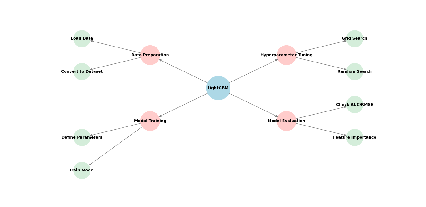
How to Use LightGBM in Python
Step 1: Import Required Libraries
import lightgbm as lgb
import numpy as np
import pandas as pd
from sklearn.model_selection import train_test_split
from sklearn.metrics import accuracy_score
Step 2: Load and Prepare Data
Let’s use the famous Iris dataset for classification:
from sklearn.datasets import load_iris

# Load dataset
iris = load_iris()
X, y = iris.data, iris.target

# Split data into train and test sets
X_train, X_test, y_train, y_test = train_test_split(X, y, test_size=0.2, random_state=42)
Step 3: Convert Data to LightGBM Format
LightGBM requires data in a special format called Dataset.
train_data = lgb.Dataset(X_train, label=y_train)
test_data = lgb.Dataset(X_test, label=y_test)
Step 4: Train a LightGBM Model
Define model parameters and train it.
params = {
    'objective': 'multiclass',  # Classification task
    'num_class': 3,  # Number of classes in Iris dataset
    'metric': 'multi_logloss',  # Loss function
    'boosting_type': 'gbdt',  # Gradient Boosting Decision Trees
    'learning_rate': 0.1,
    'num_leaves': 31,  # More leaves = more complex model
    'verbose': -1
}

# Train the model
model = lgb.train(params, train_data, valid_sets=[test_data], num_boost_round=100)
Step 5: Make Predictions
y_pred = model.predict(X_test)
y_pred_classes = np.argmax(y_pred, axis=1)  # Get class with highest probability
accuracy = accuracy_score(y_test, y_pred_classes)

print(f"Model Accuracy: {accuracy:.2f}")
LightGBM trains fast and delivers high accuracy!
LightGBM vs XGBoost – Which One is Better?
| Feature | LightGBM | XGBoost |
|---|---|---|
| Speed | 🚀 Faster | ⏳ Slower |
| Memory Usage | ✅ Lower RAM usage | ❌ Higher RAM usage |
| GPU Support | ✅ Yes (built-in) | ✅ Yes |
| Accuracy | 🔥 High | 🔥 High |
| Handles Large Datasets | ✅ Yes | ✅ Yes |
If you need the fastest boosting library with high accuracy, LightGBM is the best choice!
LightGBM is a top Python library for machine learning, known for fast training, low memory usage, and high accuracy. It’s widely used in Kaggle competitions, finance, healthcare, and e-commerce. If you’re working with structured data, LightGBM is an important tool to boost your machine learning models!
River – Online Machine Learning for Real-Time Data
When dealing with real-time data, most traditional machine learning models struggle. They require batch training, meaning they need entire datasets upfront before making predictions. But what if your data is continuously changing, like stock prices, sensor readings, or user interactions?
That’s why we use River —a powerful tool in the world of Python libraries for machine learning.
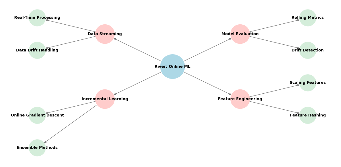
What is River?
River is a Python library for online machine learning, which means it learns from data as it arrives, one sample at a time. Unlike traditional machine learning libraries that require retraining on the entire dataset, River updates models continuously. This makes it ideal for applications where data changes in real time.
Where is River Used?
- Financial Markets – Predict stock movements as prices change
- IoT & Sensors – Monitor live data like temperature and humidity
- Fraud Detection – Analyze transactions instantly to detect fraud
- Chatbots & Recommendations – Adjust to user behavior in real time
Why Use River?
- Processes Data in Real-Time – Instead of retraining the whole model, River updates with each new data point.
- Works with Streaming Data – No need to store huge datasets; it learns on-the-fly.
- Lightweight & Efficient – Uses less memory compared to traditional models.
- Supports Classification, Regression, and Anomaly Detection – Covers a wide range of ML tasks.
Installing River
You can install River using pip:
pip install river
How to Use River in Python
Step 1: Import Required Libraries
import river
from river import datasets
from river import linear_model
from river import preprocessing
from river import metrics
Step 2: Load Streaming Data
River has built-in datasets for real-time learning. Let’s use the Airlines dataset, which tracks flight delays.
dataset = datasets.Airline()
Step 3: Define an Online Model
We’ll create a logistic regression model to predict flight delays.
model = preprocessing.StandardScaler() | linear_model.LogisticRegression()
metric = metrics.Accuracy()
StandardScaler() normalizes the data to improve model performance.| Chains the scaler and model so data flows through them.
Step 4: Train and Update the Model in Real-Time
Instead of batch training, we update the model with one sample at a time.
for x, y in dataset:
    y_pred = model.predict_one(x)  # Make a prediction
    model.learn_one(x, y)  # Update model with the new data point
    metric.update(y, y_pred)  # Update accuracy metric

print(f"Final Accuracy: {metric}")
The model continuously improves as it sees more data!
River vs. Traditional ML Libraries
| Feature | River (Online ML) | Scikit-Learn / TensorFlow (Batch ML) |
|---|---|---|
| Handles Streaming Data? | ✅ Yes | ❌ No |
| Trains on Large Datasets? | ✅ Yes (efficient) | ❌ Needs more RAM |
| Adapts to New Data? | ✅ Instantly | ❌ Needs retraining |
| Memory Usage | ✅ Low | ❌ High |
If your machine learning project involves real-time data, River is the perfect tool!
River is a game-changer in Python libraries for machine learning when working with streaming data. It’s perfect for finance, IoT, fraud detection, and recommendation systems where new data arrives constantly.
Optuna – Automatic Hyperparameter Tuning
Tuning hyperparameters is one of the most difficult and time-consuming parts of machine learning. The right settings can make your model faster, more accurate, and more efficient, but manually finding them takes a lot of time and effort.
That’s where Optuna comes in! It’s a powerful Python library that automates hyperparameter tuning, helping you find the best configurations quickly and efficiently.
What is Optuna?
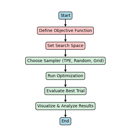
Optuna is a hyperparameter optimization library that automatically finds the best settings for your machine learning models. Instead of manually testing different values, Optuna uses advanced techniques like Bayesian Optimization and Tree-structured Parzen Estimators (TPE) to search for the most effective combination.
Where Can You Use Optuna?
- Deep Learning – Optimize learning rate, batch size, and architecture
- Machine Learning – Tune hyperparameters for decision trees, SVMs, etc.
- NLP & Computer Vision – Improve transformer models, CNNs, and more
- Any ML Model – Automate hyperparameter tuning for better performance
Installing Optuna
You can install Optuna using pip:
pip install optuna
If you’re using LightGBM or XGBoost, install them together:
pip install optuna lightgbm xgboost
How to Use Optuna for Hyperparameter Tuning
Step 1: Import Required Libraries
import optuna
from sklearn.datasets import load_iris
from sklearn.model_selection import train_test_split
from sklearn.ensemble import RandomForestClassifier
from sklearn.metrics import accuracy_score
Step 2: Define the Objective Function
This function tells Optuna what to optimize.
def objective(trial):
    # Suggest values for hyperparameters
    n_estimators = trial.suggest_int("n_estimators", 10, 200)
    max_depth = trial.suggest_int("max_depth", 2, 32)

    # Load dataset
    data = load_iris()
    X_train, X_test, y_train, y_test = train_test_split(data.data, data.target, test_size=0.2)

    # Train model with suggested hyperparameters
    model = RandomForestClassifier(n_estimators=n_estimators, max_depth=max_depth)
    model.fit(X_train, y_train)

    # Evaluate performance
    y_pred = model.predict(X_test)
    accuracy = accuracy_score(y_test, y_pred)

    return accuracy  # Optuna will maximize this value
Step 3: Run the Hyperparameter Optimization
study = optuna.create_study(direction="maximize")  # We want to maximize accuracy
study.optimize(objective, n_trials=50)  # Run 50 experiments

# Print the best hyperparameters
print("Best hyperparameters:", study.best_params)
Optuna automatically selects the best hyperparameters for your model!
Optuna vs. Manual Tuning
| Feature | Optuna (Automated) | Manual Tuning |
|---|---|---|
| Speed | 🚀 Fast (Runs multiple trials automatically) | 🐢 Slow (One by one testing) |
| Efficiency | ✅ Finds best hyperparameters | ❌ Trial and error |
| Parallelization | ✅ Yes (Multiple experiments at once) | ❌ No |
| Works with Any ML Library? | ✅ Yes | ❌ Limited |
Optuna makes hyperparameter tuning effortless and efficient!
If you want to build better models in less time, Optuna is the best python tool.
Skorch – Scikit-Learn Interface for PyTorch
Deep learning is powerful, but PyTorch can sometimes feel complex—especially if you prefer the simplicity of Scikit-Learn.
What if you could get the best of both worlds?
That’s exactly what Skorch does! It’s a Scikit-Learn wrapper for PyTorch that makes training deep learning models just as easy as using Scikit-Learn.
What is Skorch?
Skorch is a high-level Python library that allows you to train PyTorch models using the simple and familiar interface of Scikit-Learn.
Key Features:
- Easy to Use – Train models with
fit()and make predictions withpredict(), just like Scikit-Learn - Full PyTorch Power – Uses native PyTorch under the hood for flexibility and performance
- Seamless Integration – Works with Scikit-Learn pipelines, cross-validation, and grid search
- Automates Training – No need to manually write training and validation loops
Why Use Skorch?
- Scikit-Learn Simplicity – Train deep learning models without dealing with PyTorch’s complex API.
- Works with Any PyTorch Model – Supports CNNs, RNNs, Transformers, and custom architectures.
- Easier Hyperparameter Tuning – Fully compatible with
GridSearchCVandRandomizedSearchCV. - Seamless Integration – Combine deep learning with Scikit-Learn’s preprocessing and feature selection tools.
Installing Skorch
You can install Skorch using pip:
pip install skorch
If you don’t have PyTorch installed, install both:
pip install skorch torch torchvision
How to Use Skorch for Deep Learning
Step 1: Import Required Libraries
import torch
import torch.nn as nn
import torch.optim as optim
from skorch import NeuralNetClassifier
from sklearn.datasets import make_classification
from sklearn.model_selection import train_test_split
from sklearn.preprocessing import StandardScaler
from sklearn.pipeline import make_pipeline
Step 2: Define a PyTorch Model
class SimpleNN(nn.Module):
    def __init__(self, input_dim):
        super(SimpleNN, self).__init__()
        self.fc1 = nn.Linear(input_dim, 16)
        self.relu = nn.ReLU()
        self.fc2 = nn.Linear(16, 2)  # 2 output classes

    def forward(self, x):
        x = self.fc1(x)
        x = self.relu(x)
        x = self.fc2(x)
        return x
Step 3: Create a Skorch Model
Skorch makes it easy to wrap this PyTorch model inside a Scikit-Learn-like interface.
net = NeuralNetClassifier(
    SimpleNN,
    module__input_dim=20,  # Pass input dimension to the model
    max_epochs=10,
    lr=0.01,
    optimizer=optim.Adam,
    criterion=nn.CrossEntropyLoss,
    device="cpu"  # Change to "cuda" if using a GPU
)
Step 4: Train the Model
# Generate synthetic data
X, y = make_classification(n_samples=1000, n_features=20, random_state=42)

# Split the dataset
X_train, X_test, y_train, y_test = train_test_split(X, y, test_size=0.2, random_state=42)

# Standardize features
scaler = StandardScaler()

# Train using Skorch + Scikit-Learn pipeline
pipeline = make_pipeline(scaler, net)
pipeline.fit(X_train, y_train)

# Evaluate the model
accuracy = pipeline.score(X_test, y_test)
print(f"Test Accuracy: {accuracy:.2f}")
Skorch vs. Regular PyTorch
| Feature | Skorch | Regular PyTorch |
|---|---|---|
| Ease of Use | ✅ Simple fit() and predict() like Scikit-Learn | ❌ Manual training loops |
| Scikit-Learn Compatibility | ✅ Yes (pipelines, cross-validation, grid search) | ❌ No |
| Hyperparameter Tuning | ✅ Works with GridSearchCV | ❌ Manual tuning required |
| Ideal for Beginners? | ✅ Yes | ❌ More complex |
Skorch makes deep learning as easy as training an SVM!
If you love Scikit-Learn but also you need the power of PyTorch, Skorch is the perfect solution. It removes the complexity of deep learning while keeping everything flexible and customizable.
PyMC – Bayesian Machine Learning Made Easy
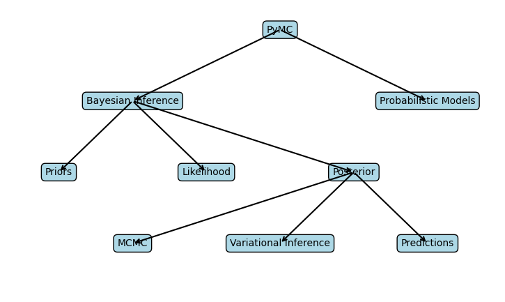
In machine learning, uncertainty is everywhere. Traditional models give a single prediction but don’t tell us how confident they are. Bayesian Machine Learning solves this by providing both predictions and a measure of uncertainty.
PyMC is one of the best Python libraries for Bayesian statistics, allowing you to build probabilistic models with just a few lines of code.
Why Use PyMC?
Traditional machine learning models predict a single value but don’t show how confident they are in that prediction. PyMC solves this by using Bayesian statistics, which gives a range of possible outcomes instead of just one answer. This is useful in finance, medicine, and research, where uncertainty matters.
Key Features:
- Handles Uncertainty – Instead of saying, “The house price is $500,000,” PyMC says, “It’s between $480,000 and $520,000 with 95% confidence.” This helps you make better decisions.
- Probabilistic Programming – You can define complex models using simple Python code, making it easy to model real-world problems with randomness.
- Automatic Inference – PyMC uses advanced Bayesian algorithms like Markov Chain Monte Carlo (MCMC) and Variational Inference to estimate the best values for your model. This means you don’t have to manually tweak parameters—it does the hard work for you.
- Built-in Visualization – PyMC includes powerful charts and graphs to help interpret results, making it easier to understand uncertainty in your predictions.
Installing PyMC
You can install PyMC using pip:
pip install pymc
If you need extra dependencies for plotting and performance optimizations, use:
pip install pymc[all]
How to Use PyMC for Bayesian Machine Learning
Let’s go step by step.
Step 1: Import Required Libraries
import pymc as pm
import numpy as np
import matplotlib.pyplot as plt
Step 2: Define a Simple Bayesian Model
Let’s say we’re estimating the probability of success for a marketing campaign. Instead of assuming a fixed percentage, we’ll model it probabilistically.
with pm.Model() as model:
    # Prior belief: Success rate follows a uniform distribution
    success_rate = pm.Beta("success_rate", alpha=2, beta=2)

    # Observed data: Out of 100 campaigns, 35 were successful
    observations = pm.Binomial("obs", n=100, p=success_rate, observed=35)

    # Run inference (estimate success rate)
    trace = pm.sample(2000, return_inferencedata=True)
PyMC automatically estimates the success rate using Bayesian inference!
Step 3: Visualize the Results
import arviz as az
az.plot_posterior(trace, var_names=["success_rate"])
plt.show()
This posterior distribution shows all possible success rates and how confident we are about them. Instead of a single number, we get a range of likely values, making our predictions more realistic and interpretable.
Where PyMC Shines
- Uncertain Data – When you’re not sure about exact values
- Small Datasets – Works well when data is limited
- Medical, Financial, and Marketing Predictions – Any field where trustworthy probability estimates matter
- A/B Testing – Compare different strategies with better confidence
PyMC vs. Traditional Machine Learning
| Feature | PyMC (Bayesian ML) | Traditional ML |
|---|---|---|
| Handles Uncertainty | ✅ Yes | ❌ No |
| Probabilistic Predictions | ✅ Yes | ❌ No |
| Works with Small Data | ✅ Yes | ❌ Needs lots of data |
| Explains Confidence in Results | ✅ Yes | ❌ No |
| Easy Hyperparameter Tuning | ✅ Uses prior knowledge | ❌ Needs trial & error |
If you want more than just predictions, PyMC is a game-changer. Instead of blindly trusting one number, it tells you how confident you should be.
AutoGluon – Automated Machine Learning (AutoML) Made Simple
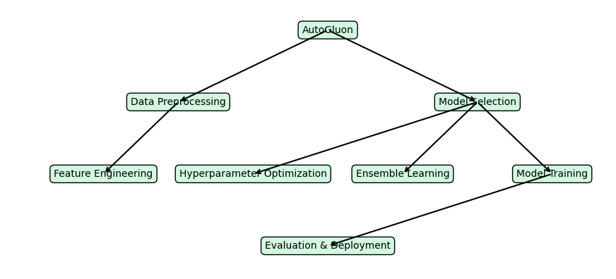
When building machine learning models, you normally have to select algorithms, tune hyperparameters, and optimize performance manually. This process takes time and requires expertise.
AutoGluon automates this entire process! It chooses the best model, tunes hyperparameters, and optimizes everything for you—all with just a few lines of code.
Why Use AutoGluon?
- No Manual Tuning – It automatically selects the best hyperparameters so you don’t have to tweak them manually.
2. Supports Multiple ML Tasks – Works for classification, regression, object detection, and text analysis without extra configuration.
3. Ensemble Learning – It combines multiple models to get better accuracy instead of relying on just one.
4. Works with Raw Data – You don’t need extensive data preprocessing—AutoGluon handles missing values and categorical features automatically.
Installing AutoGluon
You can install AutoGluon with:
pip install autogluon
For a full installation with all dependencies, use:
pip install autogluon[all]
How to Use AutoGluon for Machine Learning
Let’s go step by step and see how easy it is to train a model with AutoGluon.
Step 1: Import AutoGluon
from autogluon.tabular import TabularPredictor
import pandas as pd
Step 2: Load the Dataset
We’ll use a sample dataset to predict whether a person survives the Titanic disaster based on their characteristics.
train_data = pd.read_csv("https://autogluon.s3.amazonaws.com/datasets/Titanic/train.csv")
test_data = pd.read_csv("https://autogluon.s3.amazonaws.com/datasets/Titanic/test.csv")

# Define the target column (what we want to predict)
label = "Survived"

# Drop unnecessary columns
train_data = train_data.drop(columns=["PassengerId", "Name", "Ticket", "Cabin"])
test_data = test_data.drop(columns=["PassengerId", "Name", "Ticket", "Cabin"])
Step 3: Train the AutoML Model
AutoGluon automatically finds the best machine learning model for us.
predictor = TabularPredictor(label=label).fit(train_data)
That’s it! AutoGluon automatically trains multiple models, selects the best one, and even optimizes its hyperparameters.
Step 4: Make Predictions
Now, let’s use the trained model to predict survival on the test data.
predictions = predictor.predict(test_data)
print(predictions)
Where AutoGluon Shines
- Beginners & Experts – Perfect for those who want quick results without deep ML knowledge
- Tabular, Image, and Text Data – Works across multiple domains
- Business & Research Applications – Great for fraud detection, recommendation systems, and medical predictions
- Fast Prototyping – Quickly test ideas before fine-tuning models
AutoGluon vs. Traditional Machine Learning
| Feature | AutoGluon (AutoML) | Traditional ML |
|---|---|---|
| Model Selection | ✅ Automatic | ❌ Manual |
| Hyperparameter Tuning | ✅ Automatic | ❌ Needs trial & error |
| Works with Minimal Code | ✅ Yes | ❌ Requires detailed setup |
| Stacked Ensembling | ✅ Yes | ❌ Usually not included |
| Fast Experimentation | ✅ Yes | ❌ Takes longer |
If you want to train high-quality ML models quickly, AutoGluon is a game-changer. It automates model selection, tuning, and training, making machine learning faster and easier than ever.
Conclusion
These 8 hidden Python libraries can take your machine learning projects to the next level by making tasks easier, faster, and more efficient. Whether you’re tuning hyperparameters with Optuna, handling real-time data with River, or simplifying deep learning with Skorch, each library brings unique advantages.
By adding these tools to your workflow, you can save time, improve model performance, and handle complex ML tasks with less effort. Try them out and see how they supercharge your models!
FAQs
Why should I use these hidden Python libraries for machine learning?
Is JAX better than NumPy for machine learning?
How does AutoGluon simplify machine learning?
Can I use LightGBM instead of XGBoost?
External Resources
Here are some helpful resources to learn more about these hidden Python libraries for machine learning:
- JAX – Official Documentation
- Flax – GitHub Repository
- LightGBM – Official Documentation
- River – GitHub Repository
- Optuna – Official Documentation
- Skorch – GitHub Repository
- PyMC – Official Documentation
- AutoGluon – Official Website

")

")


Leave a Reply