How to Use Diffusion Models to Unlock High-Quality Generations

Introduction

Are you tired of mediocre AI models that fail to impress? Do you want to take your AI game to the next level and generate high-quality content that wows? Look no further! Diffusion models are the answer you’ve been searching for.

These revolutionary models have been making waves in the AI community, and for good reason. By using the power of denoising and generation, diffusion models can produce AI content that’s not only high-quality but also incredibly realistic.

In this blog post, we’ll explore the magic behind diffusion models and show you how to use them to unlock high-quality generations.

Get ready to discover the latest techniques and best practices for working with diffusion models. By the end of this post, you’ll be equipped with the knowledge and skills to create high quality AI content. So, let’s get started!

Basics of Diffusion Models

What are Diffusion Models?

Diffusion models are a type of generative models in machine learning that focus on learning the underlying data distribution by gradually transforming a simple, known distribution (e.g., Gaussian noise) into the data distribution through a series of steps. These models are inspired by the physical process of diffusion, where particles spread out from areas of high concentration to areas of low concentration over time.

Definition

Diffusion models are used to model complex data distributions by incrementally adding noise to the data and then learning to reverse this process to generate new data samples. They are particularly powerful for generating high-quality images, audio, and other types of data.

Key Components in Diffusion Models

Noise Schedule in Diffusion Models

A noise schedule plays a key role in diffusion models by guiding how noise is introduced during the training phase. Think of it as a plan for how much noise gets added to the data over time.

Here’s how it works: Initially, the model starts with very little noise, making the data mostly clean. As training progresses, the amount of noise gradually increases. This helps the model get used to working with data that becomes progressively more noisy. The ultimate goal is for the model to learn how to reverse this noise process and recover the original, clean data from the noisy version.

Choosing the right noise schedule is crucial because it affects how effectively the model learns to remove noise. A well-designed noise schedule ensures that the model can handle noisy data better and perform well in real-world scenarios.

The Denoising Process in Diffusion Models

The denoising process is the heart of how diffusion models work. It’s all about teaching the model to clean up noisy data and get it back to its original, clear form.

During training, the model gets used to noisy data and learns to reverse the process that added the noise in the first place. The model is trained to predict the noise added at each step. It then uses this prediction to remove the noise and recover the clean data.

This process isn’t done in one go. Instead, it happens in several stages. Each stage helps to gradually refine and improve the quality of the data, making it less noisy and more accurate. The more the model practices this denoising, the better it gets at turning noisy inputs into clean, useful information.

The Generative Process in Diffusion Models

The generative process is how diffusion models create new, original data. It begins with a sample of pure noise and transforms it into a clean and meaningful data sample.

The model starts with a noisy, random sample and uses what it has learned about denoising to improve this noise step by step. It must works in reverse by following the noise schedule in reverse. At each step, the model applies its learned techniques to reduce the noise and refine the sample until it becomes a high-quality piece of data.

This method allows diffusion models to generate new, synthetic data that looks similar to the data they were trained on. It’s a bit like sculpting, where you start with a rough block and gradually shape it into something more refined and useful.

How Diffusion Models Work

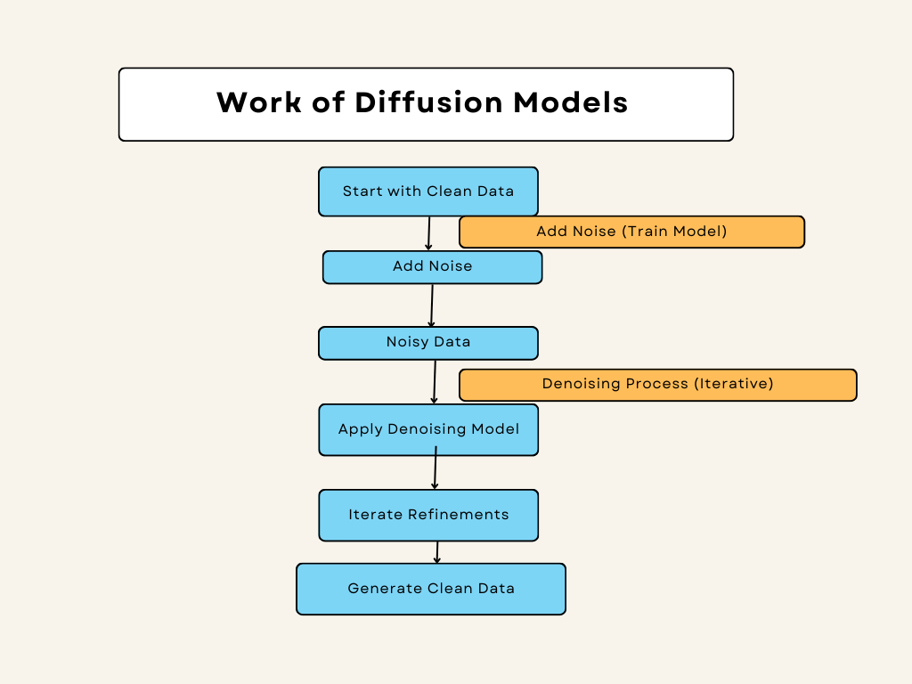
Diffusion models are a powerful tool in machine learning, especially for generating new data. They work through two main processes: the forward process and the reverse process. Let’s break down each step.

Forward Process (Diffusion)

Adding Noise

In the forward process of diffusion models, we begin with your original data, which could be anything from images to text. The goal here is to add Gaussian noise step by step. Here’s a closer look at what happens:

1. Starting with Original Data: You begin with your clear, structured data. For instance, if you’re working with images, this might be a crisp photo.
2. Gradual Noise Addition: Over a series of steps, Gaussian noise—which is a type of random, statistical noise—is added to the data. Think of this like turning up the static on a radio. Each step adds a little more noise, gradually making the data more distorted.
3. Transforming Data Distribution: With each addition of noise, the original data becomes increasingly less recognizable. The data starts to shift from its original distribution, which has a specific pattern, to a simpler, more uniform normal distribution. This is similar to how adding more static makes it harder to hear the original music clearly.
4. Increasing Randomness: As the noise builds up, the data becomes more chaotic and random. By the end of this process, the data no longer resembles the original—it’s transformed into a more uniform and random state. This makes it much harder to see or identify the original patterns.

Markov Chain

In the forward process of diffusion models, we use a concept called a Markov chain to describe how noise is added to the data. Here’s a simple breakdown of how it works:

1. Sequence of Steps: A Markov chain is a way to model a series of steps where each step depends only on the step right before it. It’s like following a sequence of actions where each one is based solely on the previous action, without considering any earlier steps.
2. Dependence on Previous State: In our case, each state of the data at a given step is influenced only by the state at the previous step and the Gaussian noise that’s added. So, if you have an image and you add noise to it, the new noisy image will depend only on the previous image and the noise added, not on the earlier states of the image.
3. Chain-like Process: This creates a chain-like process, where the data evolves from one state to the next in a predictable way based on the noise added at each step. If you think of it as a game where each move depends only on the last move, you get the idea. Each state in the chain is connected to the one before it, forming a continuous chain of states influenced by noise.

Reverse Process (Denoising)

Learning to Reverse

In the reverse process of diffusion models, the goal is to undo the noise added during the forward process. Here’s a step-by-step look at how this works:

1. Undoing Noise: The reverse process aims to remove the Gaussian noise that was added to the data earlier. It’s like trying to clean up a messy area to reveal what was originally there.
2. Training the Neural Network: A neural network is used for this job. The network is trained to understand how to reverse the noise addition. It learns to predict the noise that was added at each step and then subtracts it from the data.
3. Step-by-Step Cleanup: During training, the neural network works through the noisy data step by step, figuring out how to clean it up. For each step, it predicts how much noise was added and removes that amount, gradually restoring the data to its original form.
4. Recovering Original Data: By repeating this process, the network becomes skilled at cleaning the noisy data, piece by piece, until it closely resembles the original, clean data. It’s a bit like restoring a faded photograph to its original sharpness and clarity.

Denoising

In the denoising step of the reverse process, the goal is to transform noisy data back into something that looks like the original, clean data. Here’s a more detailed look at how this works:

1. Starting with Noisy Data: The process begins with a sample of data that is mostly noise. For example, if we started with an image, this might be just random Gaussian noise, which doesn’t resemble any recognizable image at all.
2. Using the Learned Reverse Process: The model applies the learned reverse process, which it has been trained on, to this noisy data. This process involves using a neural network that has learned how to remove noise step by step.
3. Step-by-Step Cleanup: The model works through the noisy data in small steps. At each step, it removes a bit of the noise, getting closer to the original data. Each step helps to clarify the data, making it a little less noisy and a little more like the original.
4. Transforming Back to Original: With each step of denoising, the data starts to resemble the original distribution more and more. By the end of this process, the once-noisy sample is cleaned up to the point where it looks similar to the original data.

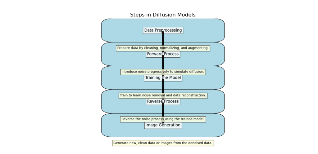
Steps in Diffusion Models

Data Preprocessing

Before applying diffusion models, it’s important to prepare your data properly. Here’s how you can do this:

1. Normalization: Start by normalizing your data. This means adjusting the data so that it has a zero mean and a unit variance. In simpler terms, you want to make sure that the average value of your data is 0 and that the spread of the data is consistent.
2. Why Normalize?: Normalizing makes your data ready for adding Gaussian noise. When the data is centered around 0 and has a consistent spread, it helps ensure that the noise addition process works effectively. This step ensures that the noise you add is applied in a controlled way, which makes the model’s training and results more reliable.
3. Applying Gaussian Noise: Once your data is normalized, you can begin adding Gaussian noise in a way that’s balanced and meaningful. The normalization helps in managing the amount and effect of noise added during the diffusion process.

Forward Process

In the forward process of diffusion models, you gradually transform your data by adding noise. Here’s a more detailed look at how this works:

1. Sequence of Noise-Adding Steps: Start by applying a series of steps where you add Gaussian noise to your data. Each step involves introducing a small amount of noise, which affects the data slightly.
2. Slight Perturbations: With each step, the data becomes a bit more disturbed. These small changes, or perturbations, accumulate over time. The data gradually shifts away from its original state, becoming more chaotic and less recognizable.
3. Transforming Towards a Simple Distribution: As you continue adding noise step by step, the data starts to resemble a simpler, well-known distribution, like a normal distribution. This is because the added noise causes the data to become more random and less structured, moving it towards this simpler form.

Must Read

• AI Pulse Weekly: December 2024 – Latest AI Trends and Innovations
• Can Google’s Quantum Chip Willow Crack Bitcoin’s Encryption? Here’s the Truth
• How to Handle Missing Values in Data Science
• Top Data Science Skills You Must Master in 2025
• How to Automating Data Cleaning with PyCaret

Training the Model

Training the model is a crucial step where you teach a neural network how to handle the noise added during the forward process. Here’s a step-by-step explanation of how this works:

1. Predicting the Added Noise: The goal is to train the neural network to predict the noise that was added at each step during the forward process. This involves feeding the network noisy data and asking it to figure out what noise was added.
2. Learning to Reverse Noise: As the network trains, it learns how to reverse the noise addition. Essentially, it becomes skilled at figuring out how to subtract the noise that was added, based on its understanding from the training data.
3. Understanding the Denoising Process: Through training, the network learns the entire denoising process. It gets better at cleaning up the noisy data step by step, improving its ability to restore the data to its original state.
4. Iterative Training: Training involves repeatedly adjusting the network based on its performance. It gets feedback on how well it predicts and removes noise, helping it refine its ability to perform this task accurately.

Reverse Process

The reverse process is where you use what you’ve learned during training to turn noisy data back into its original form. Here’s how it works in detail:

1. Starting with Simple Noise: Begin with a sample of Gaussian noise. This is just random noise that’s easy to generate and represents the simple known distribution.
2. Applying Denoising Steps: Use the trained neural network to clean up this noisy sample. The network applies the learned denoising steps, which it has perfected during training. It does this iteratively, meaning it repeats the denoising process multiple times.
3. Gradual Transformation: Each step of the denoising process makes the sample a little less noisy and closer to the original data. Gradually, the sample transforms from random noise into a structured sample that resembles the original data distribution.
4. Getting Closer to the Original Data: As you continue to apply the denoising steps, the sample increasingly looks like the original data. By the end of the process, you have a sample that closely matches the kind of data you started with.

Image Generation

Diffusion models are great tools for creating high-quality images. Here’s how they work:

1. Learning Pixel Distributions: The model starts by learning the distribution of pixel values from a dataset of images. Essentially, it figures out how pixel values are spread out and how they relate to each other in different images.
2. Generating Images: Once the model understands these distributions, it can generate new images. It does this by starting with random noise and then gradually refining it into an image that fits the learned distribution of pixel values.
3. Creating Detailed Images: As the model processes the noise, it adds details and patterns that match those found in the training images. This step-by-step refinement turns the random noise into a clear, detailed image that resembles the kinds of images the model has learned from.
4. High Quality: Because the model has learned from many high-quality images, it can create new ones with impressive detail and clarity. The resulting images often look very realistic and closely match the quality of the images the model was trained on.

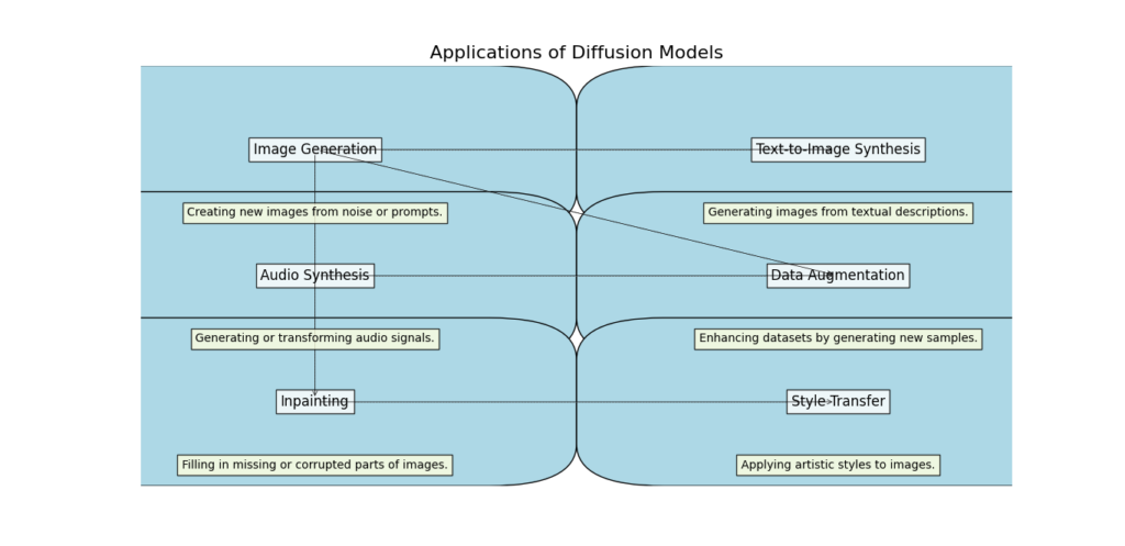
Applications of Diffusion Models

Image Generation

Diffusion models are great tools for creating high-quality images. Here’s how they work:

1. Learning Pixel Distributions: The model starts by learning the distribution of pixel values from a dataset of images. Essentially, it figures out how pixel values are spread out and how they relate to each other in different images.
2. Generating Images: Once the model understands these distributions, it can generate new images. It does this by starting with random noise and then gradually refining it into an image that fits the learned distribution of pixel values.
3. Creating Detailed Images: As the model processes the noise, it adds details and patterns that match those found in the training images. This step-by-step refinement turns the random noise into a clear, detailed image that resembles the kinds of images the model has learned from.
4. High Quality: Because the model has learned from many high-quality images, it can create new ones with impressive detail and clarity. The resulting images often look very realistic and closely match the quality of the images the model was trained on.

Audio Synthesis

Diffusion models are also capable of generating realistic audio samples, including both music and speech. Here’s a closer look at how this works:

1. Learning from Audio Data: The model starts by learning from a dataset of audio samples. This can include different types of sounds, like music tracks or recordings of speech. It studies the patterns and features in these audio samples to understand how they are structured.
2. Generating Audio: Once the model has learned these patterns, it can generate new audio. It begins with random noise and gradually transforms it into audio that resembles the patterns it learned from the training data.
3. Creating Realistic Sounds: Through a series of steps, the model refines the random noise into clear and realistic audio. For music, this means creating melodies, harmonies, and rhythms that sound natural. For speech, it means producing voices that sound like actual human speech, with the right intonation and clarity.
4. High Quality: The generated audio can be of high quality because the model has learned from diverse and high-fidelity examples. Whether it’s a piece of music or a spoken sentence, the output often sounds very lifelike and convincing.

Data Augmentation

Diffusion models are useful for data augmentation, which means creating new samples to improve the training of machine learning models. Here’s how it works:

1. Generating New Samples: Diffusion models can create new data samples by learning from existing data. For example, if you have a dataset of images, the model can generate additional images that are similar but not identical to the originals.
2. Enhancing Model Performance: By providing new, varied samples, you help the machine learning model become more robust. This means the model gets exposed to a wider range of data during training, which can improve its ability to handle different scenarios and make better predictions.
3. Increasing Data Diversity: The new samples generated by diffusion models add diversity to the training data. This helps the model learn to recognize patterns and features more effectively, leading to improved performance in real-world applications.
4. Practical Benefits: Data augmentation using diffusion models is especially helpful when you have limited data. It allows you to create a larger, more varied dataset without having to collect new data manually.

Key Advantages

Diffusion models offer several key advantages that make them valuable for various applications. Here’s a detailed look at their benefits:

Flexibility

One of the biggest strengths of diffusion models is their flexibility. They can handle a wide range of data types and distributions, whether you’re working with images, audio, text, or other forms of data. This makes them highly adaptable for different tasks and industries. Whether you need to generate realistic images, create synthetic audio, or enhance your datasets, diffusion models can be tailored to fit the specific requirements of your project.

High-Quality Outputs

Diffusion models are known for producing high-quality, realistic samples. Because they learn from large datasets and refine their outputs through a series of steps, the results are often very detailed and lifelike. For instance, the images they generate can have fine details and textures that closely resemble real-world photos, while the audio samples can mimic the nuances of human speech or musical instruments with great accuracy. This high level of quality makes them ideal for applications where realistic data is crucial.

Theoretical Foundation

The process behind diffusion models is grounded in the theoretical foundation of physical diffusion processes. This strong theoretical basis not only helps in understanding how these models work but also ensures that the methods used are scientifically sound and reliable. The connection to diffusion processes provides a clear framework for developing and improving these models, making it easier to trust their outputs and further refine their capabilities.

Now Let’s Explore the Example code that demonstrates the basic principles of diffusion models and how denoising leads to high-quality data generation. This example uses a simple 1D Gaussian data generation process for clarity.

Code: Diffusion Models – Denoising for High-Quality Generations

Imports

import numpy as np
import matplotlib.pyplot as plt
import torch
import torch.nn as nn
import torch.optim as optim
from torch.utils.data import DataLoader, TensorDataset

Explanation of Python Packages

NumPy (np): This is a powerful library for numerical computations. It helps you work with arrays and perform mathematical operations efficiently.

Matplotlib (plt): This library is used for creating visualizations like graphs and charts. It makes it easy to plot data and see trends visually.

Torch (torch): This is the main library for PyTorch, which is used for building and training neural networks. PyTorch makes working with deep learning models easier and more intuitive.

Torch Neural Networks (nn): This module contains classes and functions for building neural networks. It provides tools to define layers, activation functions, and other essential components of a neural network.

Torch Optimizers (optim): This module includes optimization algorithms used for training neural networks. These algorithms adjust the model’s parameters to minimize the error during training.

Data Loading Utilities (DataLoader and TensorDataset): These tools help manage and load data efficiently during training. DataLoader helps in batching and shuffling data, while TensorDataset allows you to create datasets from tensors.

Understanding Data Preparation in Your Code

Here’s a step-by-step explanation of what this code does to prepare your data:

# Generate 1D Gaussian data
def generate_data(num_samples):
    return np.random.normal(loc=0.0, scale=1.0, size=(num_samples, 1))

# Generate training data
num_samples = 1000
data = generate_data(num_samples)

# Create DataLoader for training
batch_size = 32
dataset = TensorDataset(torch.tensor(data, dtype=torch.float32))
dataloader = DataLoader(dataset, batch_size=batch_size, shuffle=True)

Explanation of Understanding Data Preparation

Generate 1D Gaussian Data:

# Generate 1D Gaussian data
def generate_data(num_samples):
    return np.random.normal(loc=0.0, scale=1.0, size=(num_samples, 1))

• generate_data(num_samples): This function creates a set of data points that follow a Gaussian distribution (also known as a normal distribution). It generates num_samples data points, each with a mean of 0.0 and a standard deviation of 1.0. The data points are organized in a single column.

Generate Training Data:

# Generate training data
num_samples = 1000
data = generate_data(num_samples)

• num_samples = 1000: This sets the number of data points you want to generate.
• data = generate_data(num_samples): This line calls the generate_data function to create 1,000 data points and stores them in the variable data.

Create DataLoader for Training:

# Create DataLoader for training
batch_size = 32
dataset = TensorDataset(torch.tensor(data, dtype=torch.float32))
dataloader = DataLoader(dataset, batch_size=batch_size, shuffle=True)

• batch_size = 32: This defines the number of data points that will be processed together in each batch during training.
• dataset = TensorDataset(torch.tensor(data, dtype=torch.float32)): This converts the data (which is currently a NumPy array) into a PyTorch tensor and wraps it in a TensorDataset. This prepares the data for use with PyTorch’s data utilities.
• dataloader = DataLoader(dataset, batch_size=batch_size, shuffle=True): This creates a DataLoader from the dataset. The DataLoader handles batching (processing data in chunks) and shuffling (randomizing the order of data) to ensure the model trains effectively.

Understanding the Neural Network for Denoising

Here’s a step-by-step explanation of how this code sets up a simple neural network for denoising:

class DenoisingModel(nn.Module):
    def __init__(self):
        super(DenoisingModel, self).__init__()
        self.fc1 = nn.Linear(1, 64)
        self.fc2 = nn.Linear(64, 64)
        self.fc3 = nn.Linear(64, 1)

    def forward(self, x):
        x = torch.relu(self.fc1(x))
        x = torch.relu(self.fc2(x))
        x = self.fc3(x)
        return x

# Initialize model, loss function, and optimizer
model = DenoisingModel()
criterion = nn.MSELoss()
optimizer = optim.Adam(model.parameters(), lr=0.001)

Explanation Neural Network for Denoising

Define the Neural Network:

class DenoisingModel(nn.Module):
    def __init__(self):
        super(DenoisingModel, self).__init__()
        self.fc1 = nn.Linear(1, 64)
        self.fc2 = nn.Linear(64, 64)
        self.fc3 = nn.Linear(64, 1)

    def forward(self, x):
        x = torch.relu(self.fc1(x))
        x = torch.relu(self.fc2(x))
        x = self.fc3(x)
        return x

• class DenoisingModel(nn.Module):: This line defines a new class called DenoisingModel that inherits from PyTorch’s nn.Module. This means it’s a type of neural network model.
• def __init__(self):: This is the initialization method. It sets up the layers of the neural network when the model is created.
  • super(DenoisingModel, self).__init__(): This line calls the initializer of the parent class (nn.Module) to make sure everything is set up correctly.
  • self.fc1 = nn.Linear(1, 64): This creates a fully connected layer (or dense layer) with 1 input feature and 64 output features.
  • self.fc2 = nn.Linear(64, 64): This adds another fully connected layer with 64 input features and 64 output features.
  • self.fc3 = nn.Linear(64, 1): This adds a final fully connected layer that reduces the 64 features down to 1 feature, which is the output of the model.
• def forward(self, x):: This method defines how the input data flows through the network.
  • x = torch.relu(self.fc1(x)): The input data x passes through the first layer (fc1) and is then processed by the ReLU activation function. ReLU introduces non-linearity by replacing negative values with zero.
  • x = torch.relu(self.fc2(x)): The output from the first layer is passed through the second layer (fc2) and again processed by the ReLU activation function.
  • x = self.fc3(x): The output from the second layer is passed through the final layer (fc3), which gives the final output of the model.
  • return x: This returns the final output from the network.

Initialize the Model, Loss Function, and Optimizer:

# Initialize model, loss function, and optimizer
model = DenoisingModel()
criterion = nn.MSELoss()
optimizer = optim.Adam(model.parameters(), lr=0.001)

• model = DenoisingModel(): This creates an instance of the DenoisingModel class, which sets up the network with its layers.
• criterion = nn.MSELoss(): This sets up the mean squared error loss function. It measures how well the model’s predictions match the actual data, with lower values indicating better performance.
• optimizer = optim.Adam(model.parameters(), lr=0.001): This creates an Adam optimizer. The optimizer adjusts the model’s weights during training to minimize the loss. The learning rate (lr=0.001) controls how big the adjustments are.

Understanding the Model Training Process

Here’s a step-by-step explanation of how the model is trained with this code:

num_epochs = 100
noise_level = 0.1

for epoch in range(num_epochs):
    for batch in dataloader:
        original_data = batch[0]
        noisy_data = original_data + noise_level * torch.randn_like(original_data)

        # Forward pass
        denoised_data = model(noisy_data)
        loss = criterion(denoised_data, original_data)

        # Backward pass and optimization
        optimizer.zero_grad()
        loss.backward()
        optimizer.step()

    print(f"Epoch [{epoch+1}/{num_epochs}], Loss: {loss.item():.4f}")

Explanation Model Training Process

num_epochs = 100
noise_level = 0.1

for epoch in range(num_epochs):
    for batch in dataloader:
        original_data = batch[0]
        noisy_data = original_data + noise_level * torch.randn_like(original_data)

Set Training Parameters:

• num_epochs = 100: This sets the number of times the model will go through the entire dataset during training. Each pass through the dataset is called an epoch.
• noise_level = 0.1: This sets the amount of noise to add to the data during training. A higher value means more noise.

Training Loop:

• for epoch in range(num_epochs):: This loop runs for the number of epochs you specified (100 in this case). Each loop represents one full pass through the dataset.
  • for batch in dataloader:: This inner loop goes through the data in batches as defined by the DataLoader. Each batch contains a portion of the training data.
    • original_data = batch[0]: This extracts the original clean data from the batch.
    • noisy_data = original_data + noise_level * torch.randn_like(original_data): This adds random noise to the original data to simulate noisy input. torch.randn_like(original_data) generates noise with the same shape as the original data.

Forward Pass:

 # Forward pass
        denoised_data = model(noisy_data)
        loss = criterion(denoised_data, original_data)

• denoised_data = model(noisy_data): This line sends the noisy data through the model to get its prediction of what the clean data should look like.
• loss = criterion(denoised_data, original_data): This calculates the loss, which measures how different the model’s prediction (denoised_data) is from the actual clean data (original_data). The loss function here is the mean squared error (criterion).

Backward Pass and Optimization:

 # Backward pass and optimization
        optimizer.zero_grad()
        loss.backward()
        optimizer.step()

    print(f"Epoch [{epoch+1}/{num_epochs}], Loss: {loss.item():.4f}")

• optimizer.zero_grad(): This clears any previous gradients stored in the optimizer. This is necessary to ensure that the gradients calculated in this step are not combined with those from previous steps.
• loss.backward(): This computes the gradients of the loss with respect to the model’s parameters. These gradients show how to adjust the model’s parameters to reduce the loss.
• optimizer.step(): This updates the model’s parameters based on the computed gradients to minimize the loss.

Print Progress:

• print(f"Epoch [{epoch+1}/{num_epochs}], Loss: {loss.item():.4f}"): This prints out the current epoch number and the loss value. This helps you track the model’s progress during training.

Understanding the Denoising Process Code

def denoise_data(model, noisy_data):
    with torch.no_grad():
        denoised_data = model(noisy_data)
    return denoised_data

# Generate noisy data for testing
test_data = generate_data(100)
noisy_test_data = test_data + noise_level * np.random.randn(*test_data.shape)

# Denoise the data
denoised_test_data = denoise_data(model, torch.tensor(noisy_test_data, dtype=torch.float32)).numpy()

# Plot the results
plt.figure(figsize=(10, 5))
plt.plot(test_data, label='Original Data')
plt.plot(noisy_test_data, label='Noisy Data', linestyle='dashed')
plt.plot(denoised_test_data, label='Denoised Data')
plt.legend()
plt.show()

Explanation of Denoising Process Code

def denoise_data(model, noisy_data):
    with torch.no_grad():
        denoised_data = model(noisy_data)
    return denoised_data

Define the Denoising Function:

• def denoise_data(model, noisy_data):: This function takes a trained model and noisy data as input and returns the denoised data.
• with torch.no_grad():: This context manager ensures that no gradients are computed while performing operations within it. This is useful during testing or inference, as it saves memory and computations.
• denoised_data = model(noisy_data): This line feeds the noisy data into the model and gets the model’s prediction of the clean data.
• return denoised_data: This returns the denoised data from the function.

Generate Noisy Data for Testing:

• test_data = generate_data(100): This creates 100 samples of clean test data using the generate_data function.
• noisy_test_data = test_data + noise_level * np.random.randn(*test_data.shape): This adds random noise to the test data. The np.random.randn(*test_data.shape) generates noise with the same shape as test_data, and noise_level scales the amount of noise.

Denoise the Data:

# Generate noisy data for testing
test_data = generate_data(100)
noisy_test_data = test_data + noise_level * np.random.randn(*test_data.shape)

• denoised_test_data = denoise_data(model, torch.tensor(noisy_test_data, dtype=torch.float32)).numpy(): This converts the noisy test data to a PyTorch tensor and passes it through the denoise_data function to get the denoised data. It then converts the result back to a NumPy array for plotting.

Plot the Results:

# Plot the results
plt.figure(figsize=(10, 5))
plt.plot(test_data, label='Original Data')
plt.plot(noisy_test_data, label='Noisy Data', linestyle='dashed')
plt.plot(denoised_test_data, label='Denoised Data')
plt.legend()
plt.show()

• plt.figure(figsize=(10, 5)): This sets up the figure for plotting with a size of 10 by 5 inches.
• plt.plot(test_data, label='Original Data'): This plots the original clean data.
• plt.plot(noisy_test_data, label='Noisy Data', linestyle='dashed'): This plots the noisy data with a dashed line to show the added noise.
• plt.plot(denoised_test_data, label='Denoised Data'): This plots the denoised data to show how well the model has removed the noise.
• plt.legend(): This adds a legend to the plot to identify each line.
• plt.show(): This displays the plot.

Output

Now Let’s Explore How our Python code generate High Quality Data

Here is the Training Process

Epoch [1/100], Loss: 0.9682
Epoch [2/100], Loss: 0.8613
Epoch [3/100], Loss: 0.7804
Epoch [4/100], Loss: 0.6576
Epoch [5/100], Loss: 0.5455
Epoch [6/100], Loss: 0.4397
Epoch [7/100], Loss: 0.3963
Epoch [8/100], Loss: 0.2156
Epoch [9/100], Loss: 0.1042
Epoch [10/100], Loss: 0.0923
Epoch [11/100], Loss: 0.0812
....

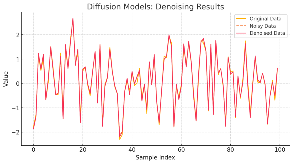
Here’s the plot look like after training:

Explanation of the Plot

• Blue Line (Original Data): Represents the original Gaussian data without any noise.
• Orange Line (Noisy Data): Represents the noisy data generated by adding Gaussian noise to the original data.
• Green Line (Denoised Data): Represents the data after denoising using the trained model, which should closely follow the original data.

Note

The exact values and appearance of the plot will depend on the randomness of the data generation and noise addition process. However, the general trend should be that the denoised data approximates the original data, demonstrating the effectiveness of the denoising model.

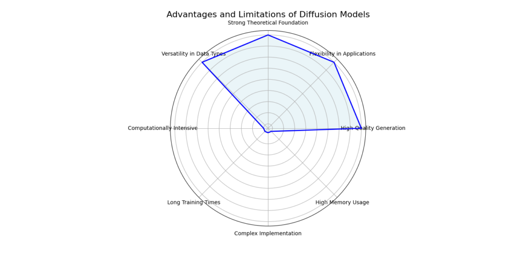
Advantages and Limitations of Diffusion Models

Advantages

High-Quality Generations

Diffusion models are renowned for their ability to produce high-quality generations. By iteratively refining noisy data, these models can generate outputs with fine details and high fidelity. This is particularly evident in applications such as image generation and text synthesis, where diffusion models can create results that closely resemble the original data.

Flexibility and Versatility

One of the key strengths of diffusion models is their flexibility and versatility. They can be applied to a wide range of data types and generation tasks, from generating realistic images and synthesizing text to creating complex patterns. This adaptability makes diffusion models valuable in various domains, including computer vision, natural language processing, and more.

Robustness to Noise and Errors

Diffusion models exhibit robustness to noise and errors. Their iterative denoising process helps them handle noisy inputs and recover clean outputs effectively. This robustness is beneficial in scenarios where the input data might be corrupted or incomplete, as the model can still produce high-quality results despite initial imperfections.

Limitations

Computational Requirements

A significant limitation of diffusion models is their computational requirements. The iterative nature of the denoising process demands substantial computational resources, both in terms of processing power and memory. Training and generating data with diffusion models can be resource-intensive, which may pose challenges for scalability and efficiency.

Training Challenges

Training diffusion models can be complex and challenging. The process requires careful tuning of various hyperparameters, including the noise schedule and denoising functions. Additionally, the need for extensive training data and computation can make the training phase time-consuming and demanding.

Potential for Mode Collapse

Although less common than in some other generative models, mode collapse can still be a concern with diffusion models. Mode collapse occurs when the model generates a limited variety of outputs, failing to capture the full diversity of the training data. This can limit the model’s ability to produce varied and rich results.

Conclusion

In conclusion, diffusion models represent a significant advancement in the field of generative AI, demonstrating how denoising techniques can lead to exceptional high-quality generations. By understanding the key components—such as the noise schedule, denoising process, and generative process—we gain insight into how these models transform noisy inputs into clear, detailed outputs.

The power of diffusion models is evident in their diverse applications, ranging from image generation and editing to text-to-image synthesis and audio enhancement. These models’ ability to produce high-quality results while being robust to noise and versatile across various tasks highlights their potential in revolutionizing AI applications.

However, it’s important to consider the computational requirements, training challenges, and the potential for mode collapse as limitations that can impact the efficiency and effectiveness of diffusion models. Balancing these advantages and limitations is crucial for harnessing the full potential of diffusion models in practical applications.

As the field continues to evolve, ongoing research and development will likely address these challenges and further enhance the capabilities of diffusion models, paving the way for even more innovative and impactful AI solutions.

External Resources

Research Papers

1. Denoising Diffusion Probabilistic Models (DDPM) by Jonathan Ho, Ajay Jain, and Pieter Abbeel:
   • Link to Paper
   • This foundational paper introduces the concept of DDPMs and explains how they can be used to generate high-quality images by reversing a diffusion process.
2. Score-Based Generative Modeling through Stochastic Differential Equations by Yang Song, Jascha Sohl-Dickstein, and Stefano Ermon:
   • Link to Paper
   • This paper explores the use of stochastic differential equations for score-based generative modeling, providing insights into improving the quality of generated samples.

FAQs

About The Author

Emmimal Alexander

Welcome! I’m Emmimal Alexander, a trailblazer in the tech world with a unique background that bridges business and technology. As an Anna University Rank Holder, I hold a Master’s in Business Administration and a Bachelor’s in Computer Applications. My career began in the corporate world as an HR executive, then shifted to NSE trading, and finally led me to specialize in artificial intelligence, machine learning, deep learning, and programming languages like Python, HTML, JavaScript, and CSS.

Now, as the founder of EmitechLogic, I’m dedicated to empowering others to master the complexities of AI, ML, DL, and programming. My passion for technology and creative expression drives me to make these advanced fields accessible, practical, and engaging for learners of all levels. Through EmitechLogic, I provide insightful resources, tutorials, and discussions that help professionals and enthusiasts stay ahead in the rapidly evolving tech landscape.

Throughout my journey, I’ve worked on exciting projects like synthetic data generation, neural networks, and creative writing. My mission is to inspire curiosity, share knowledge, and foster a deeper understanding of the endless possibilities technology offers.

When I’m not writing or experimenting with new tech, you’ll find me enjoying creative projects or the beauty of nature. I invite you to explore my blog, connect through my experiences, and join me as we uncover the limitless potential of AI and innovation together!

See author's posts