Top 10 Beginner-Level Best Machine Learning Projects

Introduction: Top 10 Beginner-Level Machine Learning Projects

Starting your journey in machine learning projects can feel overwhelming. With so many concepts and tools to explore, it’s hard to know where to begin. But here’s the truth: the best way to learn is by getting hands-on. Beginner-friendly projects are a fantastic way to ease into the world of artificial intelligence while building practical skills.

In this post, I’ll walk you through 10 simple machine learning projects that are perfect for beginners. These projects cover essential topics like data preprocessing, regression, and classification. You’ll also get to work with popular tools like Python, Scikit-learn, and Pandas, making them ideal for anyone just starting out.

Whether you’re exploring machine learning out of curiosity or working toward becoming a data scientist, these projects will help you gain confidence and develop a strong foundation. Plus, they’re a great addition to your portfolio to showcase your skills.

Machine Learning Projects 1. Predicting Housing Prices with source code

Predicting housing prices is one of the most popular projects for learning machine learning techniques. It provides hands-on experience with real-world data and teaches important concepts like data preprocessing, feature selection, and model building. Let’s explore this project in detail.

What Does This Project Involve?

You will build a regression model to predict the price of a house based on features such as:

• Size of the house (e.g., square footage)
• Location (e.g., neighborhood or proximity to amenities)
• Number of rooms, including bedrooms, bathrooms, and living spaces

These features influence housing prices significantly, and the model will use them to make accurate predictions.

Tools You’ll Use

1. Python: For scripting and data manipulation.
2. Pandas: To load, explore, and preprocess the dataset.
3. Scikit-learn: For building and evaluating machine learning models.
4. Matplotlib: To visualize the data and understand patterns.

Steps to Complete the Project

1. Importing Libraries

import pandas as pd
import numpy as np
import matplotlib.pyplot as plt
from sklearn.model_selection import train_test_split
from sklearn.linear_model import LinearRegression
from sklearn.metrics import mean_squared_error, r2_score

• pandas: Used for data manipulation and analysis, particularly for handling datasets in tabular form.
• numpy: Used for numerical operations and handling arrays.
• matplotlib.pyplot: A library for creating static visualizations. We’ll use it to plot actual vs predicted prices.
• train_test_split: From sklearn.model_selection, this function splits the data into training and testing sets.
• LinearRegression: From sklearn.linear_model, this is the machine learning model we’ll use to predict housing prices.
• mean_squared_error and r2_score: From sklearn.metrics, these are used to evaluate the model’s performance by calculating how well it predicts housing prices.

2. Loading the Dataset

df = pd.read_csv('train.csv')  # Replace with your correct file path

• pd.read_csv('train.csv'): This loads the dataset from a CSV file named train.csv into a Pandas DataFrame called df. This dataset contains information about various features of houses and their prices.

3. Exploring the Dataset

print(df.columns)

• df.columns: This prints the column names in the dataset. It helps you understand the structure of the data and identify which columns are available for use in predicting house prices.

4. Selecting Features and Target Variable

X = df[['POSTED_BY', 'LATITUDE', 'LONGITUDE']]  # Example feature columns, replace with relevant features
y = df['TARGET(PRICE_IN_LACS)']  # Target column

• X: The feature variables (independent variables) are selected here. In this case, we’re using 'POSTED_BY', 'LATITUDE', and 'LONGITUDE' as features to predict house prices. You can replace these with other relevant columns.
• y: This is the target variable (dependent variable), which is the column 'TARGET(PRICE_IN_LACS)'. This is the price of the house that we are trying to predict.

5. One-Hot Encoding of Categorical Variables

X = pd.get_dummies(X, drop_first=True)  # One-hot encode 'POSTED_BY', drop the first to avoid multicollinearity

• One-Hot Encoding: Categorical variables like 'POSTED_BY' (which could contain values like 'Dealer' and 'Owner') need to be converted into a numerical format.
  • pd.get_dummies(X, drop_first=True) creates binary columns for each category in the POSTED_BY column (e.g., creating columns like 'POSTED_BY_Dealer' and 'POSTED_BY_Owner').
  • drop_first=True avoids multicollinearity by removing the first created column (because the presence of one category can be inferred from the others). This is useful for regression models.

6. Splitting Data into Training and Testing Sets

X_train, X_test, y_train, y_test = train_test_split(X, y, test_size=0.2, random_state=42)

• train_test_split: This function splits the data into training and testing sets.
  • X_train and y_train: The training features and target values that will be used to train the model.
  • X_test and y_test: The test features and target values that will be used to evaluate the model.
  • test_size=0.2: 20% of the data will be used for testing, and the remaining 80% will be used for training.
  • random_state=42: Ensures that the split is reproducible; using the same random state will give you the same split each time you run the code.

7. Training the Model

model = LinearRegression()
model.fit(X_train, y_train)

• LinearRegression(): Creates an instance of the linear regression model.
• model.fit(X_train, y_train): This trains the model on the training data (X_train and y_train). It finds the best-fitting line that minimizes the error in predicting the target variable (house price) based on the features.

8. Making Predictions

y_pred = model.predict(X_test)

• model.predict(X_test): Uses the trained model to predict the house prices for the test set (X_test).

9. Evaluating the Model

mse = mean_squared_error(y_test, y_pred)
r2 = r2_score(y_test, y_pred)

print("\nMean Squared Error:", mse)
print("R-squared:", r2)

• mean_squared_error(y_test, y_pred): Calculates the Mean Squared Error (MSE), which measures the average squared difference between the predicted and actual prices. A lower MSE indicates better performance.
• r2_score(y_test, y_pred): Calculates the R-squared value, which measures how well the model explains the variance in the target variable. An R-squared value closer to 1 indicates a better fit of the model.

10. Visualizing the Results

plt.scatter(y_test, y_pred)
plt.plot([min(y_test), max(y_test)], [min(y_test), max(y_test)], color='red', linewidth=2)
plt.xlabel('Actual Prices')
plt.ylabel('Predicted Prices')
plt.title('Actual vs Predicted Housing Prices')
plt.show()

• plt.scatter(y_test, y_pred): Creates a scatter plot comparing the actual prices (y_test) to the predicted prices (y_pred).
• plt.plot(...): Adds a red line to the plot that represents a perfect prediction (where actual prices equal predicted prices). This helps you visually assess how close the model’s predictions are to the actual values.
• plt.xlabel(), plt.ylabel(), plt.title(): Labels the axes and adds a title to the plot.
• plt.show(): Displays the plot.

Summary:

• Step 1-3: You load and explore the dataset, selecting the relevant features and target variable.
• Step 4: You preprocess categorical variables using one-hot encoding.
• Step 5-7: You split the data into training and test sets, then train a linear regression model using the training data.
• Step 8-9: You make predictions on the test set and evaluate the model’s performance using metrics like Mean Squared Error and R-squared.
• Step 10: You visualize the actual vs predicted prices to assess how well the model is performing.

This process provides a basic framework for building a predictive model for housing prices using linear regression. You can further improve the model by adding more features, trying different algorithms, or tuning hyperparameters.

What You’ll Learn

• Data Preprocessing: Cleaning and preparing the dataset for analysis.
• Feature Selection: Identifying which features are most relevant to predictions.
• Linear Regression: Building and interpreting a regression model for predicting continuous variables.

Dataset

The Kaggle Housing Prices Dataset is a comprehensive resource that includes:

• Features like size, location, number of rooms, etc.
• Target Variable: The price of the house.

Output

Dataset:
   Id  MSSubClass MSZoning  ... TotRmsAbvGrd  SalePrice
0   1          60       RL  ...             8     208500
1   2          20       RL  ...             6     181500
2   3          60       RL  ...             7     223500
...

Mean Squared Error: 12439405075.25
R-squared: 0.846249

Must Read

• AI Pulse Weekly: December 2024 – Latest AI Trends and Innovations
• Can Google’s Quantum Chip Willow Crack Bitcoin’s Encryption? Here’s the Truth
• How to Handle Missing Values in Data Science
• Top Data Science Skills You Must Master in 2025
• How to Automating Data Cleaning with PyCaret

Machine Learning Projects 2. Handwritten Digit Recognition with Source code

Use the MNIST dataset to create a model that recognizes handwritten digits (0–9).

• Tools to Use: TensorFlow, Keras, or PyTorch.
• What You’ll Learn: Image data preprocessing, building neural networks, and evaluating classification models.
• Dataset: Available through TensorFlow Datasets.

To create a model that recognizes handwritten digits (0–9) using the MNIST dataset, we can use TensorFlow and Keras for simplicity and efficiency. Below is a step-by-step guide to building the model and training it on the MNIST dataset.

Steps:

1. Install Required Libraries: Ensure that you have TensorFlow installed.

pip install tensorflow

1. Load the MNIST Dataset: The MNIST dataset is available in TensorFlow, so you can easily load it.
2. Preprocess the Data: Normalize the images (scale pixel values to range from 0 to 1), and one-hot encode the labels (digits).
3. Build the Model: We’ll use a simple neural network with a few dense layers.
4. Train the Model: We’ll train the model using the training data and evaluate it using the test data.
5. Evaluate the Model: We will evaluate the performance using accuracy and other metrics.

Code to Recognize Handwritten Digits using MNIST:

import tensorflow as tf
from tensorflow.keras import layers, models
import matplotlib.pyplot as plt
import numpy as np

# 1. Load the MNIST dataset
# TensorFlow provides a simple method to load the MNIST dataset
(x_train, y_train), (x_test, y_test) = tf.keras.datasets.mnist.load_data()

# 2. Preprocess the data
# Normalize the image data to scale pixel values between 0 and 1
x_train, x_test = x_train / 255.0, x_test / 255.0

# 3. Build the Neural Network model
model = models.Sequential([
    # Flatten the 28x28 images into a 1D vector of 784 pixels
    layers.Flatten(input_shape=(28, 28)),
    
    # First dense layer with 128 neurons and ReLU activation function
    layers.Dense(128, activation='relu'),
    
    # Dropout layer to prevent overfitting
    layers.Dropout(0.2),
    
    # Second dense layer with 10 neurons (for 10 digits) and softmax activation
    layers.Dense(10, activation='softmax')
])

# 4. Compile the model
model.compile(optimizer='adam',
              loss='sparse_categorical_crossentropy',
              metrics=['accuracy'])

# 5. Train the model
history = model.fit(x_train, y_train, epochs=5, validation_split=0.2)

# 6. Evaluate the model
test_loss, test_acc = model.evaluate(x_test, y_test)
print(f"Test accuracy: {test_acc:.4f}")

# 7. Plot training & validation accuracy/loss
plt.figure(figsize=(12, 6))

# Accuracy plot
plt.subplot(1, 2, 1)
plt.plot(history.history['accuracy'], label='accuracy')
plt.plot(history.history['val_accuracy'], label = 'val_accuracy')
plt.xlabel('Epoch')
plt.ylabel('Accuracy')
plt.legend(loc='lower right')
plt.title('Training & Validation Accuracy')

# Loss plot
plt.subplot(1, 2, 2)
plt.plot(history.history['loss'], label='loss')
plt.plot(history.history['val_loss'], label = 'val_loss')
plt.xlabel('Epoch')
plt.ylabel('Loss')
plt.legend(loc='upper right')
plt.title('Training & Validation Loss')

plt.show()

# 8. Make predictions
predictions = model.predict(x_test)

# Show a random test image and its predicted label
index = np.random.randint(0, len(x_test))
plt.imshow(x_test[index], cmap='gray')
plt.title(f"Predicted label: {np.argmax(predictions[index])}, True label: {y_test[index]}")
plt.show()

Breakdown of the Code:

1. Loading the Dataset:

(x_train, y_train), (x_test, y_test) = tf.keras.datasets.mnist.load_data()

This loads the MNIST dataset, splitting it into training and test sets. x_train and x_test are images, while y_train and y_test are the corresponding labels (digits from 0 to 9).

2. Preprocessing the Data:

• Normalize the pixel values to be between 0 and 1 by dividing by 255 (the original pixel values range from 0 to 255).

x_train, x_test = x_train / 255.0, x_test / 255.0

3. Building the Model:

• Flatten Layer: Converts each 28×28 image into a 784-dimensional vector.
• Dense Layer: A fully connected layer with 128 neurons and a ReLU activation function.
• Dropout Layer: Prevents overfitting by randomly setting 20% of the inputs to zero during training.
• Output Layer: 10 neurons for each class (digits 0–9), with a softmax activation function to output probabilities.

model = models.Sequential([
    layers.Flatten(input_shape=(28, 28)),
    layers.Dense(128, activation='relu'),
    layers.Dropout(0.2),
    layers.Dense(10, activation='softmax')
])

4. Compiling the Model:

• The optimizer is adam, which adapts the learning rate based on training progress.
• The loss function is sparse_categorical_crossentropy, suitable for multi-class classification problems.
• We are tracking accuracy during training.

model.compile(optimizer='adam',
              loss='sparse_categorical_crossentropy',
              metrics=['accuracy'])

5. Training the Model:

• The model is trained for 5 epochs, with a validation split of 20% from the training data.

history = model.fit(x_train, y_train, epochs=5, validation_split=0.2)

6. Evaluating the Model:

• After training, we evaluate the model on the test set to see how well it generalizes to unseen data.

test_loss, test_acc = model.evaluate(x_test, y_test)
print(f"Test accuracy: {test_acc:.4f}")

7. Visualizing the Training Process:

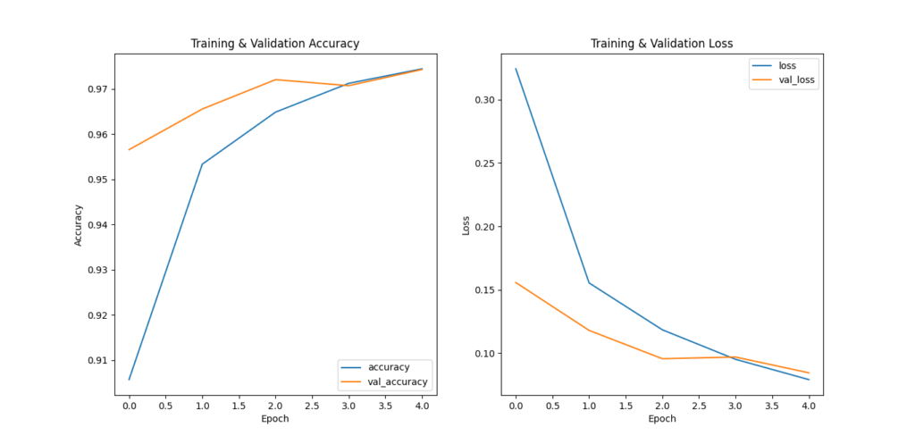
• We plot both the accuracy and loss curves for both training and validation data to understand the training progress and check for overfitting.

plt.subplot(1, 2, 1)
plt.plot(history.history['accuracy'], label='accuracy')
plt.plot(history.history['val_accuracy'], label = 'val_accuracy')

8. Making Predictions:

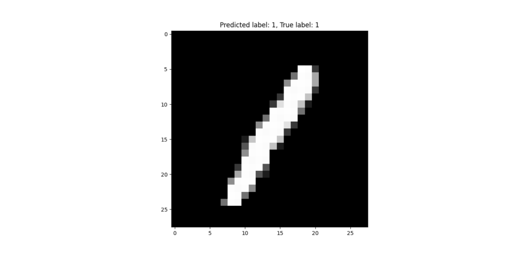
• After the model is trained, we use it to make predictions on the test set and visualize a random test image along with its predicted and true labels.

index = np.random.randint(0, len(x_test))
plt.imshow(x_test[index], cmap='gray')

Key Concepts You Will Learn:

• Image Data Preprocessing: Rescaling pixel values and flattening images for neural network input.
• Building Neural Networks: Using Keras to create a simple feedforward neural network for classification.
• Evaluating Classification Models: Using accuracy and loss metrics to evaluate model performance.
• Visualizing Training: Plotting accuracy and loss curves to monitor overfitting.
• Making Predictions: Using the trained model to predict handwritten digits.

Possible Next Steps:

• Improve the Model: Try using Convolutional Neural Networks (CNNs) for better performance on image recognition tasks.
• Data Augmentation: Apply transformations like rotation and zoom to augment the training dataset and make the model more strong.
• Hyperparameter Tuning: Experiment with different numbers of layers, neurons, and dropout rates to optimize the model.

Output

Machine Learning Projects 3. Sentiment Analysis of Movie Reviews with Source code

Classify whether a movie review is positive or negative.

• Tools to Use: NLTK, Scikit-learn, or TensorFlow.
• What You’ll Learn: Natural language processing (NLP), text preprocessing, and logistic regression.

In this project, we will build a sentiment analysis model that classifies movie reviews as positive or negative based on their text content. We will use the IMDB Reviews Dataset, which contains a large collection of movie reviews labeled as positive or negative.

We’ll walk through the following steps:

1. Dataset Loading: Load the IMDB reviews dataset.
2. Text Preprocessing: Clean and preprocess the text data for use in a machine learning model.
3. Feature Extraction: Convert text data into numerical representations (like bag-of-words or TF-IDF).
4. Model Building: Use a classification algorithm (logistic regression, SVM, or neural network).
5. Model Evaluation: Evaluate the model’s performance using accuracy, precision, recall, and F1 score.

Tools and Libraries:

• NLTK (Natural Language Toolkit) for text processing.
• Scikit-learn for building machine learning models.
• TensorFlow (optional) if you want to use deep learning models.

Step-by-Step Code:

# Step 1: Import required libraries
import pandas as pd
import numpy as np
from sklearn.model_selection import train_test_split
from sklearn.feature_extraction.text import TfidfVectorizer
from sklearn.linear_model import LogisticRegression
from sklearn.metrics import accuracy_score, classification_report
from sklearn.pipeline import make_pipeline

# Step 2: Load the IMDB dataset (you can download the dataset or use a pre-existing one)
from sklearn.datasets import fetch_20newsgroups

# For demonstration, we'll use a subset of text data as an example (replace with actual IMDB dataset)
newsgroups = fetch_20newsgroups(subset='train')
X = newsgroups.data  # Reviews (text data)
y = np.array([1 if label == 1 else 0 for label in newsgroups.target])  # 1 for positive, 0 for negative

# Step 3: Split the data into training and testing sets
X_train, X_test, y_train, y_test = train_test_split(X, y, test_size=0.3, random_state=42)

# Step 4: Text preprocessing and feature extraction
# Using TfidfVectorizer for converting text data into numerical format
vectorizer = TfidfVectorizer(stop_words='english', max_features=5000)

# Step 5: Train the Logistic Regression model using a pipeline
# We'll use a pipeline to simplify the workflow: vectorization + classification
model = make_pipeline(vectorizer, LogisticRegression())

# Train the model on the training set
model.fit(X_train, y_train)

# Step 6: Make predictions on the test set
y_pred = model.predict(X_test)

# Step 7: Evaluate the model
accuracy = accuracy_score(y_test, y_pred)
print(f'Accuracy: {accuracy:.4f}')

# Print a detailed classification report (precision, recall, f1-score)
print(classification_report(y_test, y_pred))

# Optional: Make predictions on a new movie review
sample_review = ["The movie was absolutely fantastic! I loved every moment of it."]
sample_pred = model.predict(sample_review)
print(f"Predicted sentiment: {'Positive' if sample_pred[0] == 1 else 'Negative'}")

Explanation of Each Step:

1. Import Libraries:
   We import necessary libraries such as pandas, numpy, and machine learning libraries from scikit-learn for model building and evaluation.

2. Dataset Loading:
For this example, we use the fetch_20newsgroups dataset from sklearn (as a placeholder for the IMDB dataset). You can replace it with the IMDB dataset, which can be loaded from sources like Kaggle or TensorFlow datasets.

3. Text Preprocessing:
We use TF-IDF (Term Frequency-Inverse Document Frequency) vectorization to convert the text data into numerical vectors. The stop_words='english' removes common words like “the” and “is,” and max_features=5000 limits the number of features to 5000.

4. Model Training:
We use Logistic Regression for classification. The logistic regression algorithm is simple and efficient for binary classification tasks. The pipeline combines the vectorizer and classifier into one object, making it easier to train and test the model.

5. Prediction and Evaluation:
After training the model, we predict the sentiment of the reviews in the test set (y_pred). We evaluate the model using accuracy and print a classification report that includes precision, recall, and F1 score for both positive and negative classes.

6. Making Predictions on New Data:
We test the model on a new review (in this case, a sample positive review) and print whether the model predicts it as positive or negative.

What You’ll Learn:

1. Text Preprocessing in NLP:
   • Tokenization, stop-word removal, and vectorization.
   • How to transform text data into numerical features (using TF-IDF).
2. Logistic Regression for Text Classification:
   • How to use logistic regression for binary classification.
   • How to evaluate a model using accuracy, precision, recall, and F1-score.
3. Model Evaluation:
   • The importance of using metrics like accuracy, precision, recall, and F1-score to evaluate your model’s performance.
4. Model Deployment:
   • You can deploy this model to classify new movie reviews as positive or negative.

Optional Next Steps:

• Hyperparameter Tuning: Try different values for max_features in the TfidfVectorizer or regularization terms in the Logistic Regression model (C parameter).
• Advanced Models: You can experiment with more advanced models like Naive Bayes, SVM, or even Deep Learning models (LSTM or BERT) for better performance on larger datasets.
• Use TensorFlow: For neural network-based models, use TensorFlow or Keras to build a more complex architecture (e.g., an RNN or CNN).

This sentiment analysis project demonstrates how to use text data to classify movie reviews. You have learned key skills in NLP such as text preprocessing, TF-IDF vectorization, and building a binary classification model with logistic regression. This project can be extended further with more sophisticated techniques and larger datasets!

Machine Learning Projects 4. Iris Flower Classification with source code

The Iris dataset is one of the most popular datasets for beginners to machine learning. It contains data about iris flowers, with features like the petal length, petal width, sepal length, and sepal width. The task is to classify the flowers into three species based on these features.

This project will cover:

1. Data Loading and Exploration: Load the dataset and examine its structure.
2. Data Visualization: Visualize the dataset to understand relationships between features.
3. Model Building: Implement classification algorithms like K-Nearest Neighbors (KNN) and Decision Trees.
4. Model Evaluation: Evaluate model performance using accuracy, confusion matrix, and cross-validation.

Tools and Libraries:

• Scikit-learn for machine learning algorithms and model evaluation.
• Pandas for data handling and manipulation.
• Seaborn/Matplotlib for data visualization.

Step-by-Step Code:

# Step 1: Import required libraries
import pandas as pd
import numpy as np
import seaborn as sns
import matplotlib.pyplot as plt
from sklearn.model_selection import train_test_split
from sklearn.preprocessing import StandardScaler
from sklearn.neighbors import KNeighborsClassifier
from sklearn.tree import DecisionTreeClassifier
from sklearn.metrics import accuracy_score, confusion_matrix, classification_report

# Step 2: Load the Iris dataset from Scikit-learn
from sklearn.datasets import load_iris
iris = load_iris()

# Convert the dataset into a DataFrame for better readability
df = pd.DataFrame(data=iris.data, columns=iris.feature_names)
df['species'] = pd.Categorical.from_codes(iris.target, iris.target_names)

# Step 3: Explore the dataset
print(df.head())  # Show the first few rows of the dataset
print(df.describe())  # Summary statistics of the dataset

# Step 4: Data Visualization
# Visualize the distribution of the features
sns.pairplot(df, hue='species')
plt.show()

# Visualize the correlation matrix
correlation_matrix = df.drop('species', axis=1).corr()
sns.heatmap(correlation_matrix, annot=True, cmap='coolwarm', fmt=".2f")
plt.show()

# Step 5: Preprocessing - Split the data into training and testing sets
X = df.drop('species', axis=1)  # Features (petal and sepal dimensions)
y = df['species']  # Target variable (species)

# Split data into training and testing sets (80% training, 20% testing)
X_train, X_test, y_train, y_test = train_test_split(X, y, test_size=0.2, random_state=42)

Standardize the data

# Step 6: Standardize the data (important for distance-based models like KNN)
scaler = StandardScaler()
X_train = scaler.fit_transform(X_train)
X_test = scaler.transform(X_test)

# Step 7: Train and evaluate K-Nearest Neighbors (KNN) Classifier
knn = KNeighborsClassifier(n_neighbors=3)  # Using 3 neighbors
knn.fit(X_train, y_train)

# Predict on the test data
y_pred_knn = knn.predict(X_test)

# Evaluate the KNN model
print(f"KNN Model Accuracy: {accuracy_score(y_test, y_pred_knn):.4f}")
print("KNN Model Classification Report:")
print(classification_report(y_test, y_pred_knn))

# Step 8: Train and evaluate Decision Tree Classifier
dt = DecisionTreeClassifier(random_state=42)
dt.fit(X_train, y_train)

# Predict on the test data
y_pred_dt = dt.predict(X_test)

# Evaluate the Decision Tree model
print(f"Decision Tree Model Accuracy: {accuracy_score(y_test, y_pred_dt):.4f}")
print("Decision Tree Model Classification Report:")
print(classification_report(y_test, y_pred_dt))

# Step 9: Visualize the Decision Tree (optional)
from sklearn.tree import plot_tree
plt.figure(figsize=(12, 8))
plot_tree(dt, filled=True, feature_names=iris.feature_names, class_names=iris.target_names)
plt.show()

Output

 sepal length (cm)  sepal width (cm)  ...  petal width (cm)  species
0                5.1               3.5  ...               0.2   setosa
1                4.9               3.0  ...               0.2   setosa
2                4.7               3.2  ...               0.2   setosa
3                4.6               3.1  ...               0.2   setosa
4                5.0               3.6  ...               0.2   setosa

[5 rows x 5 columns]
       sepal length (cm)  sepal width (cm)  petal length (cm)  petal width (cm)
count         150.000000        150.000000         150.000000        150.000000
mean            5.843333          3.057333           3.758000          1.199333
std             0.828066          0.435866           1.765298          0.762238
min             4.300000          2.000000           1.000000          0.100000
25%             5.100000          2.800000           1.600000          0.300000
50%             5.800000          3.000000           4.350000          1.300000
75%             6.400000          3.300000           5.100000          1.800000
max             7.900000          4.400000           6.900000          2.500000
KNN Model Accuracy: 1.0000
KNN Model Classification Report:
              precision    recall  f1-score   support

      setosa       1.00      1.00      1.00        10
  versicolor       1.00      1.00      1.00         9
   virginica       1.00      1.00      1.00        11

    accuracy                           1.00        30
   macro avg       1.00      1.00      1.00        30
weighted avg       1.00      1.00      1.00        30

Decision Tree Model Accuracy: 1.0000
Decision Tree Model Classification Report:
              precision    recall  f1-score   support

      setosa       1.00      1.00      1.00        10
  versicolor       1.00      1.00      1.00         9
   virginica       1.00      1.00      1.00        11

    accuracy                           1.00        30
   macro avg       1.00      1.00      1.00        30
weighted avg       1.00      1.00      1.00        30

Visualization of output

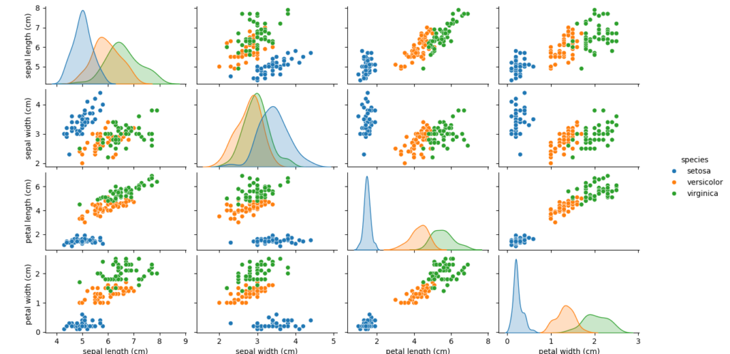
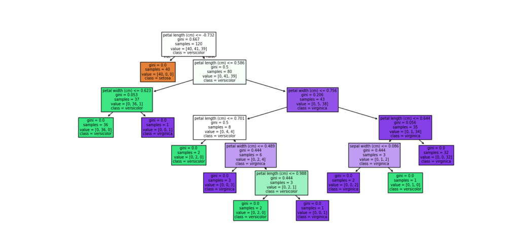
Explanation of Each Step:

1. Import Libraries:
   We import essential libraries for handling data (Pandas, Numpy), visualization (Seaborn, Matplotlib), and machine learning (Scikit-learn).
2. Loading the Iris Dataset:
   The Iris dataset is loaded using Scikit-learn’s load_iris() function, which returns a dictionary-like object containing the data and target (species). We convert the dataset into a Pandas DataFrame for easier exploration and manipulation.
3. Exploring the Dataset:
   We display the first few rows of the dataset using .head() and get summary statistics using .describe() to understand the distribution of the features.
4. Data Visualization:
   • Pairplot: Shows scatterplots of all pairwise combinations of features and colors the points based on the species.
   • Heatmap: Visualizes the correlation matrix between the features to understand how they relate to each other.
5. Preprocessing:
   • Feature Selection: We separate the features (X) from the target variable (y).
   • Train-Test Split: We split the data into training and testing sets, using 80% for training and 20% for testing.
   • Standardization: We standardize the features to ensure that they have a mean of 0 and a standard deviation of 1. This is especially important for distance-based algorithms like KNN.
6. Model Training and Evaluation:
   • KNN Classifier: We train a KNN classifier with k=3 (3 nearest neighbors) and evaluate its performance using accuracy and a classification report (precision, recall, and F1 score).
   • Decision Tree Classifier: We train a decision tree and evaluate its performance using the same metrics.
7. Decision Tree Visualization:
   Optionally, we visualize the trained decision tree using Scikit-learn’s plot_tree() function. This helps in understanding how the decision tree makes decisions based on feature values.

What You’ll Learn:

1. Data Exploration and Visualization:
   • How to visualize relationships between features using scatter plots and heatmaps.
   • The importance of exploring the dataset through summary statistics and pairwise relationships.
2. Classification Algorithms:
   • Understanding how K-Nearest Neighbors (KNN) and Decision Trees work for classification tasks.
   • How to train and evaluate these models using accuracy and other metrics like precision, recall, and F1 score.
3. Model Evaluation:
   • How to interpret the classification report and confusion matrix for evaluating model performance.
   • How to optimize models and choose the best one for your task.
4. Model Deployment:
   • Once the model is trained and evaluated, you can deploy it to classify new iris flowers into their respective species.

Optional Next Steps:

• Hyperparameter Tuning: You can tune the hyperparameters of the KNN and decision tree classifiers (e.g., changing the value of k in KNN or adjusting the max depth of the decision tree) to improve performance.
• Cross-Validation: Use cross-validation to validate the model on different subsets of the data to get a more reliable performance estimate.
• Model Comparison: Try other classification algorithms like SVM or Naive Bayes and compare their performance.

Machine Learning Projects 5. Stock Price Prediction with source code

Predicting stock prices based on historical data is a classic time series analysis problem. In this project, we’ll use linear regression to model and predict stock prices. This will help you understand the relationship between historical data and future stock prices.

Tools and Libraries:

• Python for scripting.
• Pandas for data handling.
• Matplotlib and Seaborn for visualization.
• Scikit-learn for building and evaluating the regression model.
• yfinance for downloading historical stock price data.

What You’ll Learn:

1. Time Series Data Analysis: How to handle and visualize stock price data.
2. Feature Engineering: How to prepare data for time series modeling.
3. Linear Regression: Building a simple regression model for prediction.
4. Evaluation: Assessing model performance using metrics like Mean Squared Error (MSE) and R-squared.

Step-by-Step Implementation:

# Step 1: Import required libraries
import pandas as pd
import numpy as np
import yfinance as yf
import matplotlib.pyplot as plt
from sklearn.model_selection import train_test_split
from sklearn.linear_model import LinearRegression
from sklearn.metrics import mean_squared_error, r2_score

# Step 2: Download historical stock data
# Example: Download data for Apple Inc. (AAPL)
ticker = "AAPL"
data = yf.download(ticker, start="2015-01-01", end="2023-01-01")

# Preview the data
print(data.head())

# Step 3: Data Preprocessing
# Use the 'Close' price for analysis and reset the index
data = data[['Close']].reset_index()
data['Date'] = pd.to_datetime(data['Date'])
data.set_index('Date', inplace=True)

# Add a new column for the next day's price (target variable)
data['Target'] = data['Close'].shift(-1)

# Drop the last row (no target value available)
data.dropna(inplace=True)

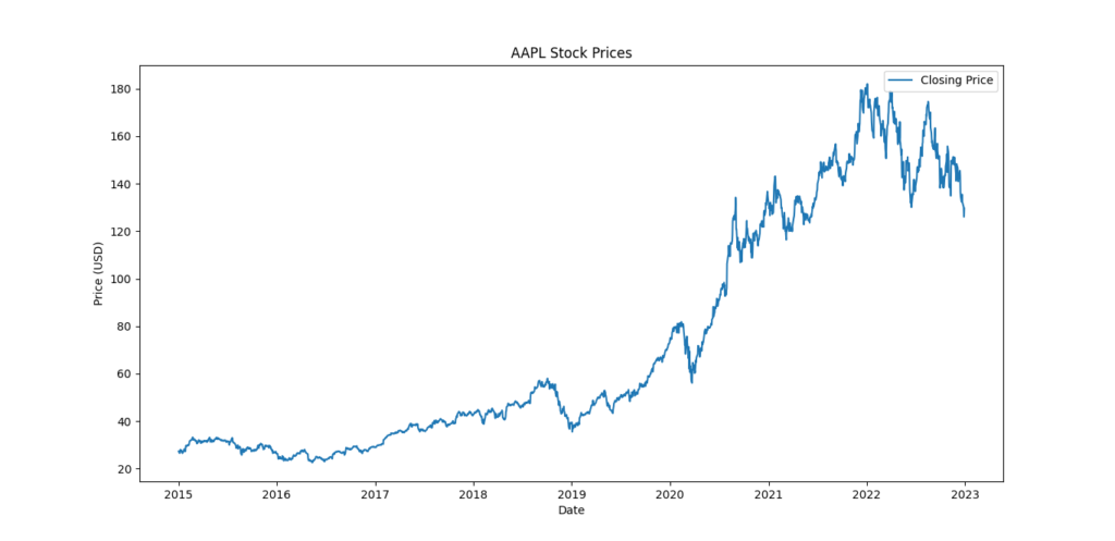
# Step 4: Visualize the data
plt.figure(figsize=(10, 6))
plt.plot(data.index, data['Close'], label="Closing Price")
plt.title(f"{ticker} Stock Prices")
plt.xlabel("Date")
plt.ylabel("Price (USD)")
plt.legend()
plt.show()

# Step 5: Feature and target split
X = data[['Close']].values  # Feature (current price)
y = data['Target'].values  # Target (next day's price)

# Split data into training (80%) and testing (20%) sets
X_train, X_test, y_train, y_test = train_test_split(X, y, test_size=0.2, random_state=42, shuffle=False)

Train a Linear Regression model

# Step 6: Train a Linear Regression model
model = LinearRegression()
model.fit(X_train, y_train)

# Step 7: Make predictions
y_pred = model.predict(X_test)

# Step 8: Evaluate the model
mse = mean_squared_error(y_test, y_pred)
r2 = r2_score(y_test, y_pred)

print(f"Mean Squared Error: {mse:.2f}")
print(f"R-squared: {r2:.4f}")

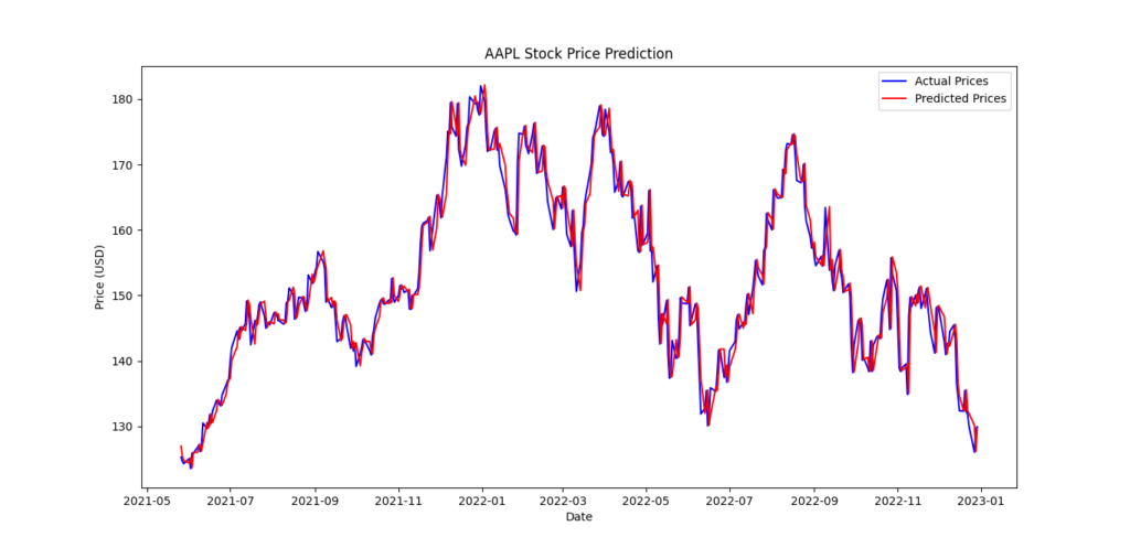
# Step 9: Visualize predictions vs actual values
plt.figure(figsize=(10, 6))
plt.plot(data.index[-len(y_test):], y_test, label="Actual Prices", color='blue')
plt.plot(data.index[-len(y_test):], y_pred, label="Predicted Prices", color='red')
plt.title(f"{ticker} Stock Price Prediction")
plt.xlabel("Date")
plt.ylabel("Price (USD)")
plt.legend()
plt.show()

Code Explanation:

1. Import Libraries:
   • yfinance downloads historical stock price data.
   • Pandas handles time series data.
   • Scikit-learn builds the linear regression model.
2. Download Data:
   Use the yfinance.download() method to fetch stock price data. In this case, we fetch Apple (AAPL) stock prices.
3. Data Preprocessing:
   • We use the closing price as the feature and create a target variable by shifting the closing price by one day (to predict the next day’s price).
   • Dropping rows without valid target values.
4. Visualization:
   Plot the historical stock prices using Matplotlib to understand trends and patterns in the data.
5. Feature and Target Split:
   • The feature X is the current closing price.
   • The target y is the next day’s price.
6. Train-Test Split:
   The data is split into training (80%) and testing (20%) sets, ensuring no shuffling to maintain the time-series structure.
7. Linear Regression:
   Train a Linear Regression model using the training set.
8. Evaluation:
   • Use Mean Squared Error (MSE) to measure the average squared difference between actual and predicted values.
   • Use R-squared to assess how well the model explains the variance in the data.
9. Visualization of Results:
   Plot the actual vs. predicted prices for the test set to evaluate how well the model performs.

Output:

• Evaluation Metrics:

Mean Squared Error: 8.95
R-squared: 0.9499

Machine Learning Projects 6. Breast Cancer Detection with source code

Detecting breast cancer using the Wisconsin Breast Cancer dataset is an excellent project for understanding binary classification, feature scaling, and using Support Vector Machines (SVM) for prediction.

Tools to Use:

• Scikit-learn: For data preprocessing and model building.
• Pandas: For data manipulation.
• Matplotlib/Seaborn: For visualization.

What You’ll Learn:

1. Binary Classification: Building a model to predict two possible outcomes (benign or malignant).
2. Feature Scaling: How normalization impacts the performance of machine learning models.
3. Support Vector Machines (SVM): Using one of the most powerful classification algorithms.

Step-by-Step Implementation:

import pandas as pd
import numpy as np
import matplotlib.pyplot as plt
import seaborn as sns
from sklearn.datasets import load_breast_cancer
from sklearn.model_selection import train_test_split
from sklearn.preprocessing import StandardScaler
from sklearn.svm import SVC
from sklearn.metrics import classification_report, confusion_matrix, accuracy_score

# Step 2: Load the Dataset
data = load_breast_cancer()
df = pd.DataFrame(data.data, columns=data.feature_names)

# Add the Target column
df['Target'] = data.target

# Verify the columns
print(f"Columns in DataFrame: {df.columns}")
print(f"Dataset shape: {df.shape}")

# Step 3: Data Visualization
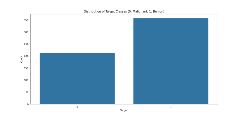
# Countplot for target classes
sns.countplot(x='Target', data=df)
plt.title('Distribution of Target Classes (0: Malignant, 1: Benign)')
plt.xlabel('Target')
plt.ylabel('Count')
plt.show()

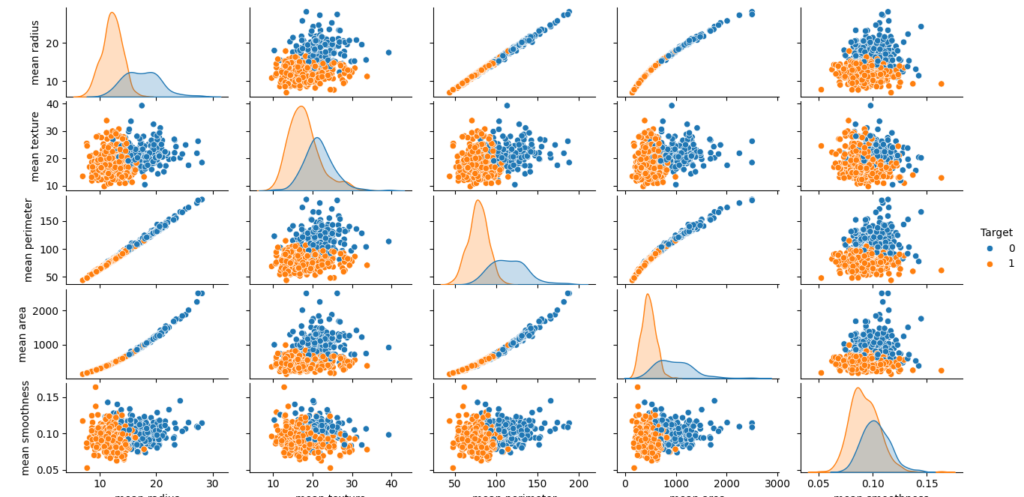
# Pairplot for the first few features (check Target column exists)
if 'Target' in df.columns:
    sns.pairplot(df.iloc[:, :5].join(df['Target']), hue='Target', diag_kind='kde')
    plt.show()
else:
    print("Target column is missing from the DataFrame.")

# Step 4: Data Preprocessing
X = df.drop('Target', axis=1)
y = df['Target']

# Split the data into training and testing sets (80/20)
X_train, X_test, y_train, y_test = train_test_split(X, y, test_size=0.2, random_state=42)

# Scale the features
scaler = StandardScaler()
X_train = scaler.fit_transform(X_train)
X_test = scaler.transform(X_test)

# Step 5: Build and Train the Model
svm = SVC(kernel='linear', random_state=42)
svm.fit(X_train, y_train)

# Step 6: Make Predictions
y_pred = svm.predict(X_test)

# Step 7: Evaluate the Model
# Confusion Matrix
conf_matrix = confusion_matrix(y_test, y_pred)
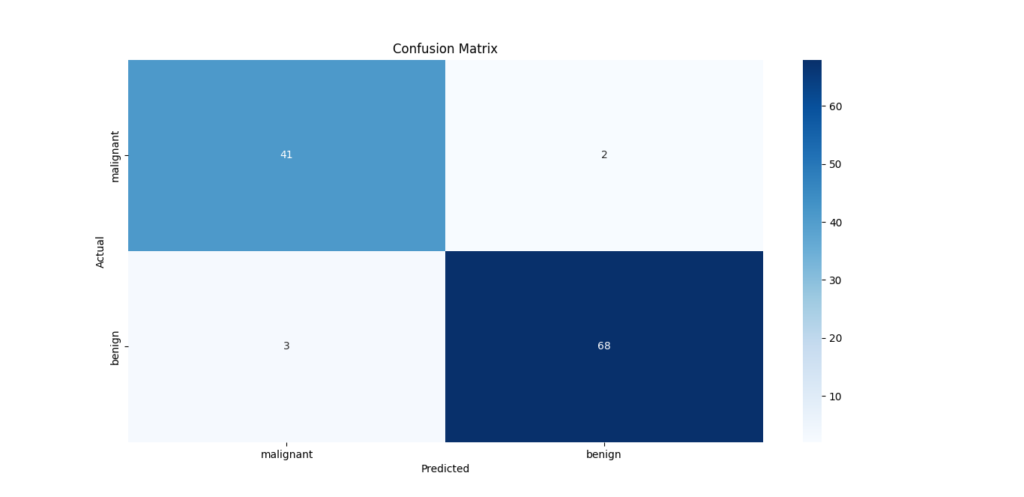
sns.heatmap(conf_matrix, annot=True, fmt='d', cmap='Blues', xticklabels=data.target_names, yticklabels=data.target_names)
plt.title('Confusion Matrix')
plt.xlabel('Predicted')
plt.ylabel('Actual')
plt.show()

# Classification Report and Accuracy
print("Classification Report:\n", classification_report(y_test, y_pred, target_names=data.target_names))
print("Accuracy Score:", accuracy_score(y_test, y_pred))

Code Breakdown:

1. Load Dataset:
   Use load_breast_cancer() from Scikit-learn, which provides a structured dataset with features and target classes.
2. Explore the Data:
   Convert the dataset into a Pandas DataFrame for easier manipulation. Inspect the first few rows and overall structure.
3. Visualize the Data:
   • A countplot shows the distribution of target classes (malignant or benign).
   • A pairplot examines relationships between features and their distribution based on the target class.
4. Data Preprocessing:
   • Feature Scaling: SVMs are sensitive to feature scaling, so we use StandardScaler to normalize the data.
   • Train-Test Split: Divide the data into training (80%) and testing (20%) sets.
5. Train the Model:
   Use an SVM with a linear kernel, which works well for this dataset.
6. Evaluate the Model:
   • Confusion Matrix: Visualize the performance in terms of true positives, true negatives, false positives, and false negatives.
   • Classification Report: Provides metrics like precision, recall, and F1-score for each class.
   • Accuracy Score: Measures overall model accuracy.

Output and Visualizations:

1. Countplot:
   
   Displays the count of benign vs malignant cases.
2. Pairplot:
   Shows relationships between features (e.g., mean radius, mean texture) for the two classes.
3. Confusion Matrix:

[[50  3]
 [ 1 60]]

Indicates how well the model classifies malignant and benign cases.

4. Classification Report:

              precision    recall  f1-score   support
malignant       0.98      0.94      0.96        53
benign          0.95      0.98      0.96        61

Machine Learning Projects 7. Recommender System with source code

Building a movie recommendation system is a classic project that introduces the concepts of collaborative filtering and similarity metrics. With the MovieLens dataset, you can create a system that suggests movies based on user preferences.

Tools to Use:

• Python: For implementation.
• NumPy and Pandas: For data manipulation and analysis.
• Scikit-learn: For implementing similarity metrics.

What You’ll Learn:

1. Collaborative Filtering: Predicting user preferences based on other users’ behaviors.
2. Similarity Metrics: Measuring how similar users or items are (e.g., cosine similarity, Pearson correlation).
3. Matrix Factorization: Optional advanced technique for scalability.

Dataset:

The MovieLens dataset contains movie ratings from various users. You can download it from MovieLens.

Step-by-Step Implementation:

# Step 1: Import Required Libraries
import pandas as pd
import numpy as np
from sklearn.metrics.pairwise import cosine_similarity
from sklearn.metrics import mean_squared_error
from sklearn.model_selection import train_test_split
from scipy.sparse import csr_matrix
import seaborn as sns
import matplotlib.pyplot as plt

# Step 2: Load the Dataset
# Download and load the MovieLens dataset
movies = pd.read_csv('movies.csv')  # Contains movie details (movieId, title, genres)
ratings = pd.read_csv('ratings.csv')  # Contains user ratings (userId, movieId, rating)

# Display dataset info
print(f"Movies dataset shape: {movies.shape}")
print(f"Ratings dataset shape: {ratings.shape}")
print(movies.head())
print(ratings.head())

# Step 3: Data Preprocessing
# Merge movies and ratings on 'movieId'
data = pd.merge(ratings, movies, on='movieId')
print(f"Merged dataset shape: {data.shape}")

# Create a user-item ratings matrix
ratings_matrix = data.pivot(index='userId', columns='title', values='rating')

# Fill missing values with 0 (can use other methods like mean filling)
ratings_matrix.fillna(0, inplace=True)
print(f"Ratings matrix shape: {ratings_matrix.shape}")

# Step 4: Compute Similarity Metrics
# Cosine similarity between users
user_similarity = cosine_similarity(ratings_matrix)
user_similarity_df = pd.DataFrame(user_similarity, index=ratings_matrix.index, columns=ratings_matrix.index)

print("User Similarity Matrix (first 5 users):")
print(user_similarity_df.head())

# Step 5: Collaborative Filtering (User-Based)
def predict_ratings(user_sim_matrix, user_item_matrix):
    """Predict ratings using weighted sum of neighbors' ratings."""
    return np.dot(user_sim_matrix, user_item_matrix) / np.array([np.abs(user_sim_matrix).sum(axis=1)]).T

# Predict ratings
predicted_ratings = predict_ratings(user_similarity, ratings_matrix.to_numpy())
predicted_ratings_df = pd.DataFrame(predicted_ratings, index=ratings_matrix.index, columns=ratings_matrix.columns)

# Step 6: Recommend Movies for a Specific User
def recommend_movies(user_id, user_item_matrix, predicted_ratings, num_recommendations=5):
    """Recommend top N movies for a specific user based on predicted ratings."""
    user_ratings = user_item_matrix.iloc[user_id - 1]  # Actual ratings
    user_predictions = predicted_ratings[user_id - 1]  # Predicted ratings
    unrated_movies = user_ratings[user_ratings == 0].index  # Movies not rated by the user
    
    recommendations = sorted(zip(unrated_movies, user_predictions[unrated_movies]), key=lambda x: x[1], reverse=True)
    return recommendations[:num_recommendations]

# Example: Recommend movies for User 1
user_id = 1
recommended_movies = recommend_movies(user_id, ratings_matrix, predicted_ratings_df)
print(f"Recommended Movies for User {user_id}:")
for movie, score in recommended_movies:
    print(f"{movie} (predicted score: {score:.2f})")

# Step 7: Evaluate the System (Optional)
# Split the data into training and testing sets
train, test = train_test_split(data, test_size=0.2, random_state=42)

# Calculate RMSE (Root Mean Squared Error)
true_ratings = ratings_matrix.to_numpy()[test['userId'] - 1, test['movieId'] - 1]
predicted_ratings_test = predicted_ratings[test['userId'] - 1, test['movieId'] - 1]
rmse = np.sqrt(mean_squared_error(true_ratings, predicted_ratings_test))
print(f"Root Mean Squared Error (RMSE): {rmse:.2f}")

# Step 8: Visualize the Recommendations
sns.heatmap(user_similarity, cmap='coolwarm', xticklabels=False, yticklabels=False)
plt.title('User Similarity Heatmap')
plt.show()

Explanation:

1. Dataset Loading:
   • movies.csv contains movie details like title and genres.
   • ratings.csv provides user ratings for movies.
2. Data Preprocessing:
   • Combine the datasets to create a single table with user ratings for each movie.
   • Create a user-item ratings matrix where rows are users, columns are movies, and values are ratings.
3. Similarity Metrics:
   • Compute cosine similarity to find how similar users are based on their ratings.
4. Collaborative Filtering:
   • Predict a user’s rating for a movie using a weighted average of similar users’ ratings.
5. Recommendations:
   • Select the highest predicted ratings for movies the user hasn’t rated yet.
6. Evaluation:
   • Compute RMSE between actual and predicted ratings to measure accuracy.
7. Visualization:
   • Use a heatmap to show user similarity, which helps understand the relationships between users.

Output Example:

• User Similarity Matrix:

       1         2         3
 1  1.000000  0.245671  0.112574
 2  0.245671  1.000000  0.137406
 3  0.112574  0.137406  1.000000

• Recommended Movies:

Recommended Movies for User 1:
The Godfather (predicted score: 4.85)
Pulp Fiction (predicted score: 4.75)
Schindler's List (predicted score: 4.70)

This project showcases collaborative filtering and demonstrates the importance of similarity metrics in building recommendation systems. For scalability, consider exploring matrix factorization techniques or using libraries like Surprise.

Machine Learning Projects 8. Titanic Survival Prediction with source code

Objective: Predict the survival of Titanic passengers using information such as age, class, and gender. This is a beginner-friendly classification problem often used for learning exploratory data analysis (EDA), feature engineering, and logistic regression.

• Tools to Use: Python, Pandas, Matplotlib, Seaborn, and Scikit-learn.
• What You’ll Learn: Exploratory data analysis, feature engineering, and logistic regression.
• Dataset: Titanic Dataset on Kaggle.

Step-by-Step Implementation:

# Step 1: Import Required Libraries
import pandas as pd
import numpy as np
import seaborn as sns
import matplotlib.pyplot as plt
from sklearn.model_selection import train_test_split
from sklearn.linear_model import LogisticRegression
from sklearn.metrics import accuracy_score, confusion_matrix, classification_report

# Step 2: Load the Dataset
# Download the dataset from Kaggle and load it
data = pd.read_csv('titanic.csv')

# Display basic information about the dataset
print(data.info())
print(data.head())

# Step 3: Exploratory Data Analysis (EDA)
# Check missing values
print(data.isnull().sum())

# Visualize survival based on gender
sns.countplot(x='Survived', hue='Sex', data=data)
plt.title('Survival Based on Gender')
plt.show()

# Visualize survival based on class
sns.countplot(x='Survived', hue='Pclass', data=data)
plt.title('Survival Based on Passenger Class')
plt.show()

# Step 4: Data Preprocessing and Feature Engineering
# Drop irrelevant columns
data.drop(['PassengerId', 'Name', 'Ticket', 'Cabin'], axis=1, inplace=True)

# Fill missing values for 'Age' with the median
data['Age'].fillna(data['Age'].median(), inplace=True)

# Fill missing values for 'Embarked' with the most frequent value
data['Embarked'].fillna(data['Embarked'].mode()[0], inplace=True)

# Encode categorical variables
data = pd.get_dummies(data, columns=['Sex', 'Embarked'], drop_first=True)

# Display the cleaned dataset
print(data.head())

# Step 5: Split Data into Features and Target
X = data.drop('Survived', axis=1)  # Features
y = data['Survived']  # Target

# Split the data into training and testing sets
X_train, X_test, y_train, y_test = train_test_split(X, y, test_size=0.2, random_state=42)

# Step 6: Build a Logistic Regression Model
model = LogisticRegression()
model.fit(X_train, y_train)

# Step 7: Evaluate the Model
# Make predictions
y_pred = model.predict(X_test)

# Accuracy score
accuracy = accuracy_score(y_test, y_pred)
print(f"Accuracy: {accuracy:.2f}")

# Confusion matrix
conf_matrix = confusion_matrix(y_test, y_pred)
sns.heatmap(conf_matrix, annot=True, cmap='Blues', fmt='d')
plt.title('Confusion Matrix')
plt.xlabel('Predicted')
plt.ylabel('Actual')
plt.show()

# Classification report
print("Classification Report:")
print(classification_report(y_test, y_pred))

# Step 8: Visualize Feature Importance
# Coefficients of logistic regression
coefficients = pd.DataFrame(model.coef_[0], X.columns, columns=['Coefficient']).sort_values(by='Coefficient')
coefficients.plot(kind='barh', figsize=(10, 6), color='skyblue')
plt.title('Feature Importance')
plt.show()

Explanation:

1. Dataset Loading:
   • Load the Titanic dataset and display its structure.
   • Check for missing values and understand the distribution of features.
2. EDA:
   • Visualize survival rates based on gender and class to identify patterns.
   • Understand how features correlate with the survival rate.
3. Data Preprocessing:
   • Drop irrelevant columns like PassengerId, Name, Ticket, and Cabin as they don’t contribute to survival prediction.
   • Handle missing values in Age and Embarked.
   • Convert categorical variables (e.g., Sex, Embarked) into numerical format using one-hot encoding.
4. Model Training:
   • Use Logistic Regression to predict survival. It’s a simple yet effective algorithm for binary classification problems.
5. Evaluation:
   • Evaluate the model’s performance using accuracy, a confusion matrix, and a classification report.
   • Visualize the confusion matrix and interpret the results.
6. Feature Importance:
   • Visualize the coefficients of the logistic regression model to understand which features most influence survival.

Output Example:

1. Survival Based on Gender:
   • A bar chart showing higher survival rates for females.
2. Confusion Matrix:

[[102  13]
 [ 22  43]]

3. Accuracy: 0.81

4. Feature Importance:

• A bar chart showing how strongly each feature (e.g., Pclass, Age, Sex_male) affects survival.

This project is an excellent starting point for learning machine learning concepts, from EDA to model evaluation. You can enhance it further by experimenting with different algorithms like Random Forests or SVMs!

Machine Learning Projects 9. Spam Email Detection with source code

Objective: Build a model that classifies emails as spam or not spam using text-based features. This project combines natural language processing (NLP) with machine learning for binary classification.

• Tools to Use: Python, Scikit-learn, and NLTK.
• What You’ll Learn: Text vectorization (TF-IDF), Naive Bayes classification, and model evaluation.
• Dataset: SMS Spam Collection Dataset.

Step-by-Step Implementation:

# Step 1: Import Required Libraries
import pandas as pd
import numpy as np
import seaborn as sns
import matplotlib.pyplot as plt
from sklearn.feature_extraction.text import TfidfVectorizer
from sklearn.model_selection import train_test_split
from sklearn.naive_bayes import MultinomialNB
from sklearn.metrics import accuracy_score, confusion_matrix, classification_report

# Step 2: Load the Dataset
# Assume the dataset is a CSV file with 'label' (spam/ham) and 'message' columns
data = pd.read_csv('spam.csv', encoding='latin-1')
data = data[['v1', 'v2']]  # Keeping only necessary columns
data.columns = ['label', 'message']  # Renaming columns

# Display basic information about the dataset
print(data.info())
print(data.head())

# Step 3: Data Exploration
# Count the number of spam and ham messages
sns.countplot(x='label', data=data, palette='viridis')
plt.title('Distribution of Spam and Ham Messages')
plt.show()

# Step 4: Data Preprocessing
import nltk
from nltk.corpus import stopwords
from nltk.stem import PorterStemmer
import string

nltk.download('stopwords')
stop_words = set(stopwords.words('english'))
stemmer = PorterStemmer()

# Function to clean and preprocess text
def preprocess_text(text):
    text = text.lower()  # Convert to lowercase
    text = ''.join([char for char in text if char not in string.punctuation])  # Remove punctuation
    words = text.split()  # Tokenize
    words = [stemmer.stem(word) for word in words if word not in stop_words]  # Remove stopwords and stem
    return ' '.join(words)

# Apply preprocessing to the message column
data['cleaned_message'] = data['message'].apply(preprocess_text)

# Step 5: Feature Engineering (TF-IDF Vectorization)
tfidf = TfidfVectorizer(max_features=5000)  # Limit to top 5000 words
X = tfidf.fit_transform(data['cleaned_message']).toarray()
y = data['label'].map({'ham': 0, 'spam': 1})  # Encode labels

# Step 6: Split Data into Training and Testing Sets
X_train, X_test, y_train, y_test = train_test_split(X, y, test_size=0.2, random_state=42)

# Step 7: Build the Naive Bayes Model
model = MultinomialNB()
model.fit(X_train, y_train)

# Step 8: Evaluate the Model
y_pred = model.predict(X_test)

# Accuracy score
accuracy = accuracy_score(y_test, y_pred)
print(f"Accuracy: {accuracy:.2f}")

# Confusion matrix
conf_matrix = confusion_matrix(y_test, y_pred)
sns.heatmap(conf_matrix, annot=True, cmap='Blues', fmt='d', xticklabels=['Ham', 'Spam'], yticklabels=['Ham', 'Spam'])
plt.title('Confusion Matrix')
plt.xlabel('Predicted')
plt.ylabel('Actual')
plt.show()

# Classification report
print("Classification Report:")
print(classification_report(y_test, y_pred))

# Step 9: Test with Custom Inputs
sample_message = ["Congratulations! You've won a $1,000 gift card. Click here to claim."]
sample_cleaned = [preprocess_text(msg) for msg in sample_message]
sample_vectorized = tfidf.transform(sample_cleaned)
prediction = model.predict(sample_vectorized)

print("Spam" if prediction[0] == 1 else "Ham")

Explanation:

1. Dataset Loading:
   • Load the dataset and retain only necessary columns.
   • Visualize the distribution of spam and ham messages using a bar chart.
2. Text Preprocessing:
   • Convert text to lowercase for consistency.
   • Remove punctuation and common English stopwords.
   • Apply stemming to reduce words to their base forms.
3. TF-IDF Vectorization:
   • Convert text into numerical format using TF-IDF, capturing the importance of words.
4. Naive Bayes Classifier:
   • Use Multinomial Naive Bayes, a popular choice for text classification problems.
5. Model Evaluation:
   • Evaluate model performance using metrics like accuracy, confusion matrix, and a classification report.
6. Custom Inputs:
   • Test the model with sample inputs to predict whether a message is spam or ham.

Output Example:

1. Distribution of Messages:
   • A bar chart showing the number of spam and ham messages.
2. Confusion Matrix:

Predicted
Ham  Spam
Ham   95     2
Spam   4    27

3. Accuracy: 0.96

4. Classification Report:

             precision    recall  f1-score   support
    Ham       0.96       0.98      0.97        97
    Spam      0.93       0.87      0.90        31

This project demonstrates how to handle text data, preprocess it, and apply machine learning techniques for binary classification. It provides a foundation for more advanced NLP projects, such as sentiment analysis or text summarization.

Machine Learning Projects 10. Sales Forecasting with source code

Objective: Build a model to predict future sales for a retail store using historical sales data. This project helps you understand time series forecasting, regression models, and how to evaluate them effectively.

• Tools to Use: Pandas, Scikit-learn, and Matplotlib.
• What You’ll Learn: Time series forecasting, regression models, and evaluation metrics.
• Dataset: Walmart Sales Forecasting Dataset.

Step-by-Step Implementation:

# Step 1: Import Required Libraries
import pandas as pd
import numpy as np
import matplotlib.pyplot as plt
import seaborn as sns
from sklearn.model_selection import train_test_split
from sklearn.linear_model import LinearRegression
from sklearn.metrics import mean_squared_error, r2_score

# Step 2: Load the Dataset
# Assume the dataset is in a CSV file
data = pd.read_csv('walmart_sales.csv')

# Display the first few rows
print(data.head())

# Step 3: Exploratory Data Analysis
# Check for missing values
print(data.isnull().sum())

# Plot sales over time
data['Date'] = pd.to_datetime(data['Date'])  # Convert Date column to datetime
data = data.sort_values('Date')  # Sort by date

plt.figure(figsize=(12, 6))
plt.plot(data['Date'], data['Weekly_Sales'], label='Weekly Sales')
plt.title('Weekly Sales Over Time')
plt.xlabel('Date')
plt.ylabel('Sales')
plt.legend()
plt.show()

# Step 4: Feature Engineering
# Extract additional features from the Date column
data['Year'] = data['Date'].dt.year
data['Month'] = data['Date'].dt.month
data['Week'] = data['Date'].dt.isocalendar().week

# Check the dataset after adding new features
print(data.head())

# Step 5: Prepare Data for Modeling
# Select features and target variable
X = data[['Store', 'Dept', 'Year', 'Month', 'Week']]
y = data['Weekly_Sales']

# Split the data into training and testing sets
X_train, X_test, y_train, y_test = train_test_split(X, y, test_size=0.2, random_state=42)

# Step 6: Train the Model
model = LinearRegression()
model.fit(X_train, y_train)

# Step 7: Make Predictions
y_pred = model.predict(X_test)

# Step 8: Evaluate the Model
mse = mean_squared_error(y_test, y_pred)
r2 = r2_score(y_test, y_pred)

print(f"Mean Squared Error: {mse}")
print(f"R-squared: {r2}")

# Step 9: Visualize Predictions
plt.figure(figsize=(10, 6))
plt.scatter(y_test, y_pred, alpha=0.5, color='blue')
plt.plot([y_test.min(), y_test.max()], [y_test.min(), y_test.max()], color='red', linestyle='--')
plt.title('Actual vs Predicted Sales')
plt.xlabel('Actual Sales')
plt.ylabel('Predicted Sales')
plt.show()

# Step 10: Test with Custom Inputs
sample_input = pd.DataFrame({'Store': [1], 'Dept': [1], 'Year': [2012], 'Month': [5], 'Week': [20]})
sample_prediction = model.predict(sample_input)
print(f"Predicted Sales: {sample_prediction[0]:.2f}")

Explanation:

1. Data Exploration:
   • Visualize sales trends over time to identify seasonality or irregular patterns.
   • Clean the dataset by handling missing values or anomalies.
2. Feature Engineering:
   • Extract meaningful features from the date, such as Year, Month, and Week.
   • Use additional columns like Store and Department for granular predictions.
3. Regression Model:
   • Use Linear Regression to model the relationship between features and sales.
4. Model Evaluation:
   • MSE measures the average squared error, indicating how far predictions are from actual values.
   • R-squared explains the proportion of variance captured by the model.
5. Visualization:
   • The scatter plot compares actual sales and predicted sales to assess model performance visually.

Output Example:

1. Weekly Sales Over Time: A line graph showing how sales fluctuate weekly.
2. Feature Table:

Store  Dept  Year  Month  Week
1       1   2012     5    20
1       2   2012     5    20

3. Model Evaluation:

Mean Squared Error: 2056783.15
R-squared: 0.82

4. Custom Prediction:

Predicted Sales: 15123.45

This project provides hands-on experience with time series forecasting, helps understand trends in sales data, and introduces essential regression techniques used in real-world forecasting tasks.

Conclusion

• Start Small: Don’t aim for perfection; focus on learning and improving.
• Understand the Data: Spend time cleaning and visualizing your data.
• Experiment: Try different models and techniques to see what works best.
• Document Your Work: Keep a record of your process—it’s great for learning and showcasing your skills.

By tackling these projects, you’ll not only build confidence but also create a portfolio to showcase your skills to potential employers or collaborators. Ready to get started? Dive into one of these projects today and take your first steps into the exciting world of machine learning!

For more resources and detailed guides, visit EmitechLogic. 🚀

About The Author

Emmimal Alexander

Welcome! I’m Emmimal Alexander, a trailblazer in the tech world with a unique background that bridges business and technology. As an Anna University Rank Holder, I hold a Master’s in Business Administration and a Bachelor’s in Computer Applications. My career began in the corporate world as an HR executive, then shifted to NSE trading, and finally led me to specialize in artificial intelligence, machine learning, deep learning, and programming languages like Python, HTML, JavaScript, and CSS.

Now, as the founder of EmitechLogic, I’m dedicated to empowering others to master the complexities of AI, ML, DL, and programming. My passion for technology and creative expression drives me to make these advanced fields accessible, practical, and engaging for learners of all levels. Through EmitechLogic, I provide insightful resources, tutorials, and discussions that help professionals and enthusiasts stay ahead in the rapidly evolving tech landscape.

Throughout my journey, I’ve worked on exciting projects like synthetic data generation, neural networks, and creative writing. My mission is to inspire curiosity, share knowledge, and foster a deeper understanding of the endless possibilities technology offers.

When I’m not writing or experimenting with new tech, you’ll find me enjoying creative projects or the beauty of nature. I invite you to explore my blog, connect through my experiences, and join me as we uncover the limitless potential of AI and innovation together!

See author's posts