Unlocking New Potentials: Data Augmentation with Generative AI

Introduction

In the fast-paced world of machine learning and deep learning, having a large and varied dataset is crucial. But collecting enough diverse data can be a real challenge. This is where data augmentation and generative AI come into play, offering creative solutions to these problems.

What if you could expand your dataset significantly from just a few samples? What if you could make your data more diverse and rich without spending hours collecting new samples? This is the potential of combining data augmentation with generative AI.

In this blog post, we’ll explore how these methods can transform your machine learning projects. From boosting your image datasets to creating realistic synthetic data, you’ll learn how to use these techniques to improve your model’s performance and add more flexibility to your work.

Join us as we unlock new potentials with data augmentation and generative AI, showing you how these powerful tools can make a big difference in your projects.

Overview of Generative AI and Data Augmentation

Generative AI and data augmentation are game-changers in the field of machine learning. These techniques offer powerful ways to enhance and expand datasets, which are crucial for training effective models.

Generative AI involves using algorithms to create new data that resembles your original dataset. This can include generating new images, text, or even entire datasets. Techniques like GANs (Generative Adversarial Networks) and variational autoencoders are at the forefront of this exciting technology. By creating realistic synthetic data, generative AI helps overcome the limitations of small or biased datasets.

Data augmentation, on the other hand, involves modifying existing data to create new samples. This can be as simple as flipping an image or as complex as changing the colors or adding noise. These transformations can significantly increase the diversity of your training data, making your models more accurate and generalizable.

Combining these two techniques opens up new possibilities. You can not only create entirely new data with generative AI but also enhance and expand it further with data augmentation. This synergy is especially valuable in fields like computer vision, where having a vast and varied dataset is essential for success.

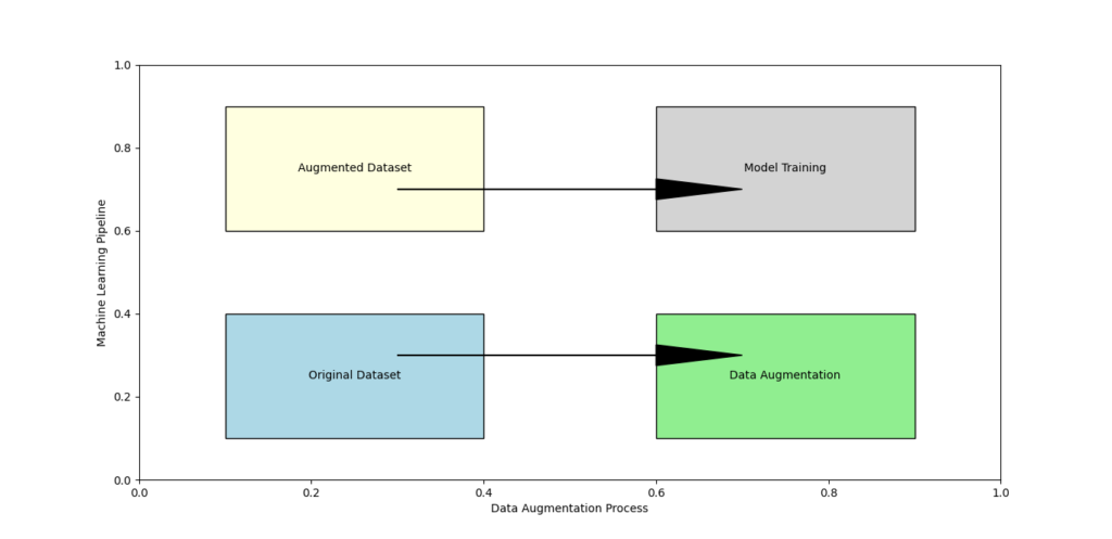
In this overview, we’ll explore how generative AI and data augmentation work, their benefits, and how you can apply them to your own projects. By the end, you’ll have a clear understanding of how these innovative methods can elevate your machine learning efforts. Here let’s see How Data Augmentation works

Importance of Data Augmentation in Machine Learning and Deep Learning

In the world of machine learning and deep learning, the quality of your data can make or break your model’s performance. However, collecting large, diverse datasets is often challenging. This is where data augmentation steps in, offering a powerful solution to enhance and expand your training data.

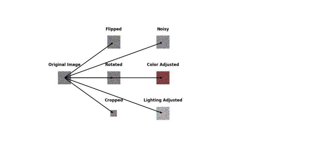
Data augmentation involves transforming existing data to create new samples. Simple techniques like rotating, flipping, or cropping images can significantly increase the size and diversity of your dataset. More advanced methods can add noise, change colors, or adjust lighting conditions, making your models more resilient to variations in real-world data.

The benefits of data augmentation go beyond just increasing dataset size. By creating varied versions of your data, you help your models learn to generalize better, leading to improved accuracy and strongness. This is especially important in fields like computer vision and natural language processing, where models need to handle a wide range of inputs and conditions.

Another key advantage is that data augmentation can help mitigate the risk of overfitting. Overfitting occurs when a model learns the training data too well, including its noise and anomalies, leading to poor performance on new, unseen data. By introducing varied and augmented data, you can help your model learn more general patterns, reducing overfitting and improving its performance on real-world tasks.

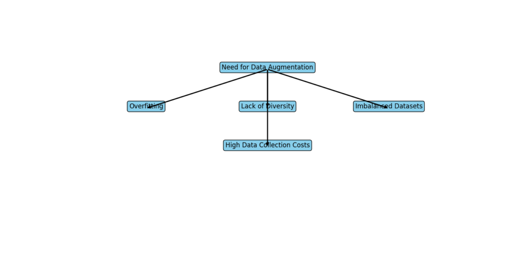
The Need for Data Augmentation

Challenges of Limited Data in Machine Learning

In machine learning, the quality and quantity of data are crucial for building effective models. However, several challenges arise when working with limited data:

Overfitting

When a model is trained on a small dataset, it tends to overfit, meaning it performs well on the training data but poorly on unseen data. Overfitting occurs because the model learns the noise and details in the training data, which do not generalize to new data. This can lead to misleadingly high accuracy during training but poor performance in real-world applications.

Lack of Diversity

Limited data often lacks diversity, making it difficult for the model to learn the full range of possible variations. This leads to poor performance in real-world applications where the data can vary significantly from the training set. For example, if a facial recognition system is trained only on images of young people, it might not perform well on images of older adults or people from different ethnic backgrounds.

Imbalanced Datasets

Many datasets are imbalanced, with some classes having significantly more samples than others. This imbalance can bias the model towards the majority class, resulting in poor performance on the minority class. For instance, in medical diagnostics, if the dataset has more healthy images than diseased ones, the model might become biased towards predicting the healthy class, missing critical diagnoses.

High Data Collection Costs

Collecting large and diverse datasets can be expensive and time-consuming. This is especially true in fields like medical imaging and autonomous driving, where acquiring labeled data requires significant resources and expertise. In medical imaging, each labeled image might need to be reviewed by a specialist, while in autonomous driving, collecting diverse driving scenarios involves significant logistical challenges.

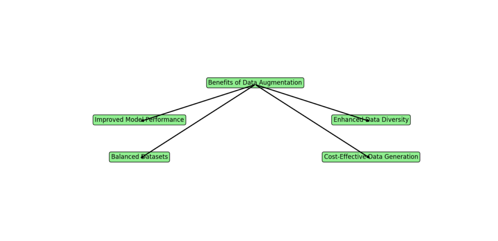
Benefits of Data Augmentation

Data augmentation addresses the challenges of limited data by artificially increasing the size and diversity of the training dataset. Here are some key benefits:

Improved Model Performance

By augmenting the training data, models can learn from a more diverse set of examples, leading to better generalization and performance on unseen data. This helps reduce the risk of overfitting. For instance, a model trained on augmented data might perform better in various conditions because it has encountered a wider range of scenarios during training.

Enhanced Data Diversity

Data augmentation techniques create variations in the existing data, introducing new examples that the model can learn from. This increased diversity helps the model become more adaptable to variations in real-world data. For example, rotating, flipping, or cropping images can provide different perspectives, making the model more adept at recognizing objects in different orientations and backgrounds.

Balanced Datasets

Data augmentation can generate additional samples for underrepresented classes, helping to balance the dataset. This leads to more fair and accurate models that perform well across all classes. In a classification task with imbalanced data, generating synthetic examples for the minority class ensures the model doesn’t become biased toward the majority class.

Cost-Effective Data Generation

Data augmentation provides a cost-effective way to increase the size of the training dataset without the need for expensive data collection. This is particularly beneficial in domains where data is scarce or difficult to obtain. For example, in medical imaging, augmenting existing images can significantly reduce the need for new, manually labeled images, saving both time and resources.

Real-World Examples of Data Augmentation

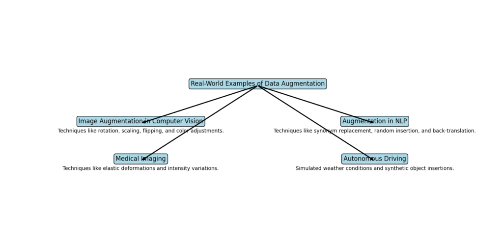
Image Augmentation in Computer Vision

In computer vision, data augmentation is widely used to improve model performance. Techniques such as rotation, scaling, flipping, and color adjustments are applied to existing images to create new training samples. For example, in object detection tasks, these augmented images help the model learn to recognize objects from different angles and in various lighting conditions. This means a model trained with augmented data can better identify objects whether they are partially obstructed, rotated, or displayed under various lighting conditions.

Augmentation in Natural Language Processing (NLP)

In natural language processing (NLP), data augmentation techniques like synonym replacement, random insertion, and back-translation are used to generate new text samples. These techniques help models become more adaptable to different phrasing and language variations. For instance, in sentiment analysis, augmenting the text data with different expressions of the same sentiment helps the model understand various ways of expressing positive or negative sentiments. This means a sentiment analysis model can accurately detect sentiment even if the phrasing changes, improving its overall performance.

Medical Imaging

In medical imaging, acquiring labeled data is often challenging due to the need for expert annotations. Data augmentation techniques, such as elastic deformations and intensity variations, are used to generate new medical images from existing ones. This helps improve the performance of models used for tasks like tumor detection and organ segmentation. By augmenting the data, the model can learn to identify tumors or organs even when they appear slightly different in shape or intensity from the training images.

Autonomous Driving

In the field of autonomous driving, collecting diverse training data covering all possible driving scenarios is impractical. Data augmentation techniques, such as simulated weather conditions and synthetic object insertions, are used to create a more comprehensive training dataset. This helps improve the performance and safety of autonomous driving systems. For example, by simulating rain, fog, or different traffic conditions, the model can learn to navigate safely under various scenarios, enhancing the reliability of autonomous vehicles.

Must Read

• AI Pulse Weekly: December 2024 – Latest AI Trends and Innovations
• Can Google’s Quantum Chip Willow Crack Bitcoin’s Encryption? Here’s the Truth
• How to Handle Missing Values in Data Science
• Top Data Science Skills You Must Master in 2025
• How to Automating Data Cleaning with PyCaret

How Data Augmentation works

Common Data Augmentation Techniques

Enhancing your datasets with data augmentation techniques is a powerful way to improve the performance of your machine learning models. Here’s a detailed look at some popular methods for augmenting image, text, and audio data.

1. Image Data Augmentation

a. Geometric Transformations

• Rotation: This technique involves rotating the image by a certain angle. For instance, turning an image of a cat by 45 degrees can help the model recognize the cat regardless of its orientation.
• Translation: Shifting the image horizontally or vertically. Moving an image of a dog 10 pixels to the right can help the model recognize the dog even if it’s not centered.
• Scaling: Enlarging or shrinking the image. Doubling the size of an image of a car can help the model identify the car at various scales.
• Flipping: Flipping the image horizontally or vertically. Flipping an image of a tree horizontally can help the model learn to identify the tree from different perspectives.
• Shearing: Slanting the shape of the image. Applying a shear transformation to an image of a building can simulate different angles and perspectives.

b. Color Space Transformations

• Brightness Adjustment: Changing the brightness of the image. For example, increasing the brightness of a photo taken in a dim room can help the model handle variations in lighting.
• Contrast Adjustment: Modifying the contrast of the image. Enhancing contrast can make the edges in a photo more pronounced, aiding the model in edge detection.
• Saturation Adjustment: Changing the saturation of colors in the image. Increasing saturation can make the colors more vivid, helping the model distinguish between different objects.
• Hue Adjustment: Altering the hue of the image. Shifting the hue can change the overall color tone, making a sunset photo appear more orange, for example.

c. Noise Injection

• Gaussian Noise: Adding random Gaussian noise to the image. This technique can simulate the effect of poor lighting conditions or low-quality cameras.
• Salt and Pepper Noise: Adding random white and black pixels to the image. This method mimics sensor noise and can help the model become more resilient to such disturbances.

d. Cropping and Padding

• Random Cropping: Cropping a random part of the image can focus on different parts of the image, enhancing the model’s ability to generalize.
• Padding: Adding padding around the image can provide more context. For instance, adding a white border around an image of a cat can create more varied training examples.

Here is an image demonstrating how data augmentation works. Starting with an original image, data augmentation creates a horizontally flipped version, rotates the image by 90 degrees, and crops a portion of the image.

Example: Image Data Augmentation using Keras

Here is an example of how to apply image data augmentation using the Keras library:

from tensorflow.keras.preprocessing.image import ImageDataGenerator
from tensorflow.keras.datasets import cifar10
import matplotlib.pyplot as plt

# Load CIFAR-10 dataset
(x_train, y_train), (x_test, y_test) = cifar10.load_data()

# Create an ImageDataGenerator object
datagen = ImageDataGenerator(
    rotation_range=40,
    width_shift_range=0.2,
    height_shift_range=0.2,
    shear_range=0.2,
    zoom_range=0.2,
    horizontal_flip=True,
    fill_mode='nearest'
)

# Fit the data generator on the training data
datagen.fit(x_train)

# Generate augmented images
augmented_images = datagen.flow(x_train, y_train, batch_size=1)

# Display some augmented images
for i in range(9):
    plt.subplot(330 + 1 + i)
    batch = next(augmented_images)
    image = batch[0].astype('uint8')
    plt.imshow(image[0])
plt.show()

Explanation:

• ImageDataGenerator: Creates a generator for real-time data augmentation.
• rotation_range, width_shift_range, height_shift_range, shear_range, zoom_range, horizontal_flip, fill_mode: Parameters to apply different types of transformations.
• fit: Computes necessary statistics on the training data (e.g., mean and standard deviation).
• flow: Generates batches of augmented images.

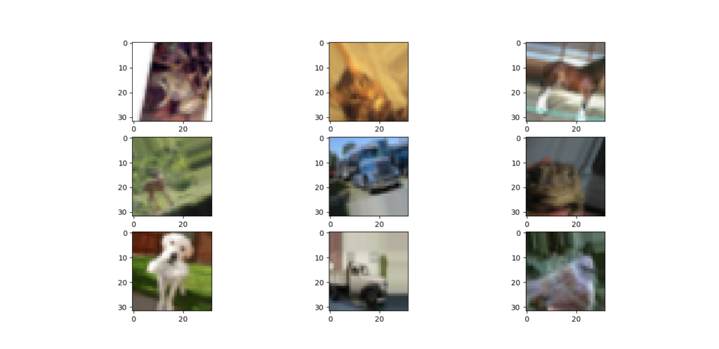
Here’s the Output

Output Explanation

Grid of Images:

• The output will be a matplotlib figure with a 3×3 grid of images.
• Each cell in the grid will contain an augmented image from the CIFAR-10 dataset.

• Image 1: A CIFAR-10 image of a cat, rotated 15 degrees.
• Image 2: A CIFAR-10 image of a truck, shifted to the right by 5%.
• Image 3: A CIFAR-10 image of a bird, zoomed in by 10%.
• And so on, with each image showing a different augmentation effect.

2. Text Data Augmentation

a. Synonym Replacement

Replacing words with their synonyms to create variations in text. For example, swapping “happy” with “joyful” in a sentence can help the model understand different expressions of the same concept.

b. Random Insertion

Inserting random words into the text. Adding words like “suddenly” into a sentence can change its context, helping the model learn to handle unexpected additions.

c. Random Deletion

Deleting random words from the text can simplify sentences and teach the model to understand shorter versions of text.

d. Random Swap

Swapping the positions of random words in the text. For instance, changing “blue sky” to “sky blue” can help the model learn different syntactic structures.

Example: Text Data Augmentation using Keras

Data augmentation is not only beneficial for images but also for text data. In text data augmentation, we generate new text samples by applying various transformations to the original text. These transformations can include synonym replacement, random insertion, random swap, and random deletion. This process helps to create a more robust model by providing diverse training examples.

Here is an example of text data augmentation using Keras and the nlpaug library, which is a popular tool for natural language processing (NLP) data augmentation.

Step-by-Step Implementation

1: Install Required Libraries

First, you need to install the nlpaug library if you haven’t already:

pip install nlpaug

2: Import Libraries

import nlpaug.augmenter.word as naw
import numpy as np
import tensorflow as tf
from tensorflow.keras.preprocessing.text import Tokenizer
from tensorflow.keras.preprocessing.sequence import pad_sequences
from tensorflow.keras.models import Sequential
from tensorflow.keras.layers import Embedding, LSTM, Dense, Dropout

3: Sample Text Data

texts = [
    "I love machine learning.",
    "Data augmentation is very useful.",
    "Natural Language Processing is a fascinating field.",
    "Deep learning models require a lot of data.",
    "Text data augmentation can improve model performance."
]
labels = [1, 1, 1, 1, 1]  # Sample labels for demonstration

4: Text Data Augmentation

We will use the nlpaug library to augment the text data. In this example, we will use synonym replacement augmentation.

# Define the augmenter
aug = naw.SynonymAug(aug_src='wordnet')

# Apply augmentation
augmented_texts = []
for text in texts:
    augmented_texts.append(aug.augment(text))

# Combine original and augmented texts
all_texts = texts + augmented_texts
all_labels = labels * 2  # Duplicate labels for augmented data

5: Text Preprocessing

Tokenize and pad the text sequences.

# Tokenize the text
tokenizer = Tokenizer()
tokenizer.fit_on_texts(all_texts)
sequences = tokenizer.texts_to_sequences(all_texts)

# Pad the sequences
maxlen = 10
X = pad_sequences(sequences, maxlen=maxlen)
y = np.array(all_labels)

6: Define and Train the Model

Define a simple LSTM model and train it on the augmented dataset.

# Define the model
model = Sequential([
    Embedding(input_dim=len(tokenizer.word_index) + 1, output_dim=50, input_length=maxlen),
    LSTM(64),
    Dropout(0.5),
    Dense(1, activation='sigmoid')
])

# Compile the model
model.compile(optimizer='adam', loss='binary_crossentropy', metrics=['accuracy'])

# Train the model
model.fit(X, y, epochs=10, batch_size=2)

Explanation

1. Install Required Libraries: The nlpaug library is used for text data augmentation.
2. Import Libraries: Necessary libraries for NLP, augmentation, and Keras are imported.
3. Sample Text Data: A small set of example sentences is provided.
4. Text Data Augmentation: Synonym replacement is applied to each sentence using nlpaug. This creates augmented versions of the original text.
5. Text Preprocessing: The text is tokenized and padded to ensure uniform input length for the model.
6. Define and Train the Model: A simple LSTM model is defined, compiled, and trained on the augmented dataset.

Output

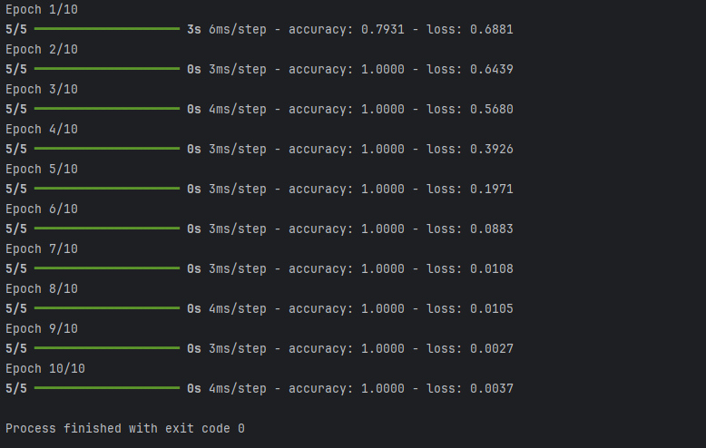
The output will show the training process of the model, including the loss and accuracy for each epoch. Since we are using a small dataset and a simple model, this example primarily demonstrates the process of text data augmentation and how it can be integrated into a Keras-based workflow.

By augmenting text data, we can effectively increase the diversity and size of the training dataset, which helps improve the model’s ability to generalize to new, unseen data.

Summary

• The model achieved perfect accuracy early in the training process and maintained it throughout all epochs.
• The loss consistently decreased, indicating that the model was learning effectively from the augmented data.
• The quick convergence to perfect accuracy suggests that the dataset was likely small and simple, allowing the model to learn patterns quickly.

3. Audio Data Augmentation

a. Time Stretching

Changing the speed of the audio without altering its pitch. For example, making a song play faster while keeping the same notes can help the model handle different playback speeds.

b. Pitch Shifting

Changing the pitch of the audio without affecting its speed. This technique can make a voice sound higher or lower, helping the model recognize different pitches.

c. Adding Noise

Adding random noise to the audio signal can simulate the effect of background noise, making the model more robust to noisy environments.

d. Time Shifting

Shifting the audio signal in time can help the model handle different starting points in the audio.

e. Volume Adjustment

Increasing or decreasing the volume of the audio can help the model learn to recognize sounds at different volumes.

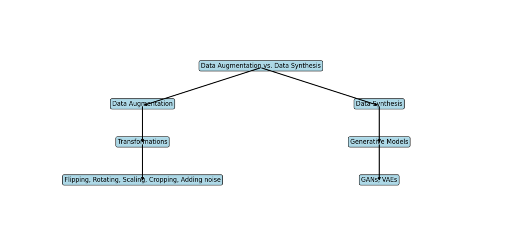
Data Augmentation vs. Data Synthesis

In the realm of machine learning and deep learning, the terms data augmentation and data synthesis are often mentioned. Both are crucial techniques for enhancing datasets, but they serve different purposes and are used in distinct ways.

Data Augmentation

Data augmentation is the process of creating new data samples from existing data. This is done by applying various transformations to the original data, such as:

• Flipping: Horizontally or vertically flipping images.
• Rotating: Rotating images by a certain angle.
• Scaling: Zooming in or out.
• Cropping: Extracting random patches from images.
• Adding noise: Introducing random variations.

These transformations help increase the size and diversity of the training data, making models more strong and better at generalizing to new, unseen data. Data augmentation is particularly effective in computer vision tasks, where slight variations in the input can significantly improve model performance.

Data Synthesis

Data synthesis, on the other hand, involves generating entirely new data samples that do not exist in the original dataset. This is achieved using generative models such as:

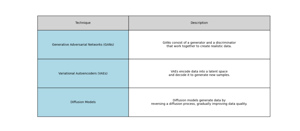
• GANs (Generative Adversarial Networks): These models consist of two networks, a generator and a discriminator, that work together to produce realistic synthetic data.
• Variational Autoencoders (VAEs): These models learn to encode data into a latent space and then decode it back to generate new samples.

Data synthesis is particularly useful when the available dataset is small or lacks diversity. For example, in medical imaging, where obtaining labeled data can be difficult and expensive, synthetic data can provide a valuable supplement. Additionally, data synthesis can create entirely new scenarios or conditions that may be rare or difficult to capture in the real world.

Key Differences

• Source: Data augmentation relies on existing data, applying transformations to create new samples. Data synthesis generates new data from scratch using generative models.
• Complexity: Data augmentation techniques are generally simpler and computationally less intensive. Data synthesis requires training complex models like GANs or VAEs.
• Use Cases: Data augmentation is widely used in tasks like image classification and object detection to enhance existing datasets. Data synthesis is used when there is a need for entirely new data, such as creating rare disease samples in medical research.

Comparison of Generative AI Techniques for Data Augmentation

Generative Adversarial Networks (GANs)

Structure of GANs

Overview

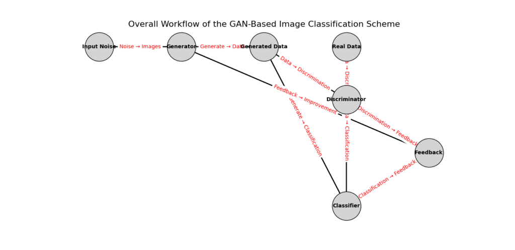
Generative Adversarial Networks (GANs) consist of two main components: the generator and the discriminator. These two neural networks engage in a process known as adversarial training, where they compete against each other to improve the quality of the generated data. This competitive framework is the core of GANs’ ability to produce realistic and high-quality data samples.

The Generator

The generator is a neural network responsible for creating new data samples. It takes in random noise as input and transforms it into data that mimics the real dataset. The generator’s goal is to produce data that is indistinguishable from the actual data, effectively “fooling” the discriminator.

1. Input Layer: The generator starts with a layer that accepts a random noise vector, typically sampled from a standard normal distribution. This noise vector serves as a seed for generating new data.
2. Hidden Layers: These layers consist of several layers of neurons, often utilizing techniques such as transposed convolutions (also known as deconvolutions) to upsample the input noise into a higher-dimensional space. These layers progressively refine the noise into more structured and detailed data representations.
3. Output Layer: The final layer outputs data that has the same dimensions as the real data. For image generation, this could be a 2D grid of pixels representing an image.

The Discriminator

The discriminator is a neural network that evaluates the authenticity of data samples. It takes in both real data and data generated by the generator and aims to distinguish between the two.

1. Input Layer: The discriminator receives a data sample, either from the real dataset or from the generator.
2. Hidden Layers: These layers are designed to extract features from the input data. In the case of image data, convolutional layers are commonly used to identify patterns and textures that help in distinguishing real images from fake ones.
3. Output Layer: The final layer outputs a single value, typically between 0 and 1, representing the probability that the input data is real. A value close to 1 indicates high confidence that the data is real, while a value close to 0 indicates high confidence that the data is generated.

Adversarial Training

The training process of GANs involves the generator and discriminator competing in a zero-sum game:

1. Generator Training: The generator generates a batch of fake data samples and sends them to the discriminator. The discriminator evaluates these samples alongside real data and provides feedback on their authenticity. The generator’s loss function is designed to maximize the discriminator’s error, effectively training the generator to produce more realistic data over time.
2. Discriminator Training: The discriminator is trained to correctly classify real and fake data. Its loss function is designed to minimize the classification error, improving its ability to distinguish between real and generated samples.
3. Iterative Process: The generator and discriminator are trained alternately in an iterative process. As the generator becomes better at producing realistic data, the discriminator becomes more adept at identifying subtle differences between real and fake data, leading to continuous improvement in both networks.

Strengths of GANs

High-Quality Data

GANs can generate highly realistic data samples, making them ideal for applications like image generation and style transfer. The generator network learns to create data that closely resembles the real data, while the discriminator network learns to distinguish between real and generated data. Over successive training iterations, the generator improves its ability to produce high-quality, realistic samples that can be used to enhance the training dataset. For example, GANs can produce detailed and accurate synthetic images that can be used to augment datasets in computer vision tasks.

Wide Range of Data Types

GANs can be applied to a wide range of data types, including images, text, and audio. This flexibility makes them useful in various fields. In text generation, GANs can create coherent and contextually appropriate sentences. In audio synthesis, GANs can produce realistic speech or music samples. This ability to generate diverse types of data allows GANs to be employed in numerous applications, from artificial intelligence research to practical industry solutions.

Limitations of GANs

Training Complexity

Training GANs can be challenging due to the adversarial nature of the process, which requires careful balancing of the generator and discriminator. The two networks are trained simultaneously in a competitive setting: the generator aims to produce data that can fool the discriminator, while the discriminator strives to correctly identify real versus fake data. This can lead to issues like mode collapse, where the generator produces limited variations of data, or unstable training, where the networks fail to converge. Fine-tuning hyperparameters and implementing advanced training techniques are often necessary to achieve stable and effective training.

Resource Intensive

GANs often require significant computational resources and time to train effectively. The training process involves numerous iterations where both networks are updated repeatedly, demanding substantial processing power and memory. High-performance GPUs or TPUs are typically needed to handle the computational load. Additionally, the training duration can be lengthy, especially for complex tasks or large datasets, making it resource-intensive. This can limit the accessibility of GANs for individuals or organizations with limited computational capabilities.

Practical Applications of GANs in Data Augmentation

Generative Adversarial Networks (GANs) have emerged as a powerful tool for data augmentation, enhancing various machine learning tasks by generating realistic and diverse data samples. Here are some practical applications of GANs in data augmentation:

Image Generation for Computer Vision

Enhancing Training Datasets

GANs can generate high-quality images that augment existing datasets, providing additional training samples for computer vision tasks. This is particularly useful in scenarios where acquiring large amounts of labeled images is challenging or expensive.

• Object Detection: GANs can create variations of objects in different poses, lighting conditions, and backgrounds, improving the strongness of object detection models.
• Facial Recognition: GANs can produce diverse facial images, helping to train more accurate facial recognition systems.

Style Transfer

GANs can be used for style transfer, where the style of one image is applied to another. This can augment datasets with images in various artistic styles, lighting conditions, and textures.

• Artistic Image Generation: By transferring the style of famous artworks to regular photos, GANs can create unique and diverse training samples for art-related applications.

Data Augmentation for Imbalanced Datasets

Addressing Class Imbalance

GANs can generate additional samples for underrepresented classes in a dataset, balancing the dataset and improving model performance.

• Medical Imaging: GANs can create synthetic images of rare diseases, providing more balanced datasets for training medical diagnostic models.
• Fraud Detection: In financial datasets where fraudulent transactions are rare, GANs can generate synthetic fraud cases to help train more effective detection models.

Text-to-Image Synthesis

Enhancing Text Descriptions with Visual Data

GANs can generate images from text descriptions, augmenting datasets where paired text and image data are needed.

• E-commerce: GANs can create product images based on text descriptions, enriching datasets for recommendation systems and visual search applications.
• Story Illustration: GANs can generate illustrations for storybooks based on textual content, providing a rich dataset for training models in creative and educational applications.

Augmenting Speech and Audio Data

Generating Synthetic Audio Samples

GANs can be used to generate synthetic audio data, which is useful for training speech recognition and audio classification models.

• Speech Recognition: GANs can produce diverse speech samples with different accents, pitches, and background noises, enhancing the strongness of speech recognition systems.
• Music Generation: GANs can create new music tracks by learning from existing music datasets, providing additional training data for music classification and recommendation models.

Real-World Example: Using GANs to Augment Images for Medical Diagnosis

In this example, we use Generative Adversarial Networks (GANs) to augment a dataset of medical images. This augmentation can improve the performance of machine learning models used for medical diagnosis by providing additional training samples.

Here’s a step-by-step implementation using the MNIST dataset as a stand-in for medical images. For actual medical images, you’ll need to replace the MNIST dataset with your medical imaging dataset.

Step-by-Step Code Explanation

Import Required Libraries

import tensorflow as tf
from tensorflow.keras.datasets import mnist
from tensorflow.keras.layers import Dense, Reshape, Flatten, Dropout, Input
from tensorflow.keras.models import Sequential
from tensorflow.keras.optimizers import Adam
import numpy as np

We start by importing necessary libraries: TensorFlow for building and training the GAN, and NumPy for data manipulation.

Load and Preprocess the Data

(x_train, _), (_, _) = mnist.load_data()
x_train = (x_train.astype('float32') - 127.5) / 127.5  # Normalize to [-1, 1]
x_train = x_train.reshape(x_train.shape[0], 28, 28)   # Reshape to add channel dimension if necessary

• Load MNIST Data: We load the MNIST dataset. For actual medical images, replace this with your dataset.
• Normalize Data: Normalize the image data to the range [-1, 1].
• Reshape Data: Reshape the data to ensure it matches the input requirements of the neural networks.

Build the Generator

generator = Sequential([
    Dense(256, input_dim=100, activation='relu'),
    Dense(512, activation='relu'),
    Dense(1024, activation='relu'),
    Dense(784, activation='tanh'),
    Reshape((28, 28))
])

The generator is responsible for creating new data samples.

• Dense Layers: Series of dense layers with ReLU activation functions to introduce non-linearity.
• Output Layer: The final dense layer outputs a vector of size 784 (28×28), reshaped into a 28×28 image with tanh activation to match the normalized range.

Verify Generator

assert generator.count_params() > 0, "Generator has no trainable weights!"

Check that the generator has trainable weights.

Build the Discriminator

discriminator = Sequential([
    Flatten(input_shape=(28, 28)),
    Dense(1024, activation='relu'),
    Dropout(0.3),
    Dense(512, activation='relu'),
    Dropout(0.3),
    Dense(256, activation='relu'),
    Dropout(0.3),
    Dense(1, activation='sigmoid')
])

The discriminator evaluates the authenticity of generated samples.

• Flatten Layer: Converts the 2D image input into a 1D vector.
• Dense Layers with Dropout: Series of dense layers with ReLU activation and dropout layers to prevent overfitting.
• Output Layer: Final dense layer outputs a single value with sigmoid activation to indicate the probability of the input being real.

Verify Discriminator

assert discriminator.count_params() > 0, "Discriminator has no trainable weights!"

Check that the discriminator has trainable weights.

Compile the Discriminator

discriminator.compile(loss='binary_crossentropy', optimizer=Adam(), metrics=['accuracy'])

Compile the discriminator with binary cross-entropy loss and Adam optimizer.

Build and Compile the GAN

discriminator.trainable = False
gan_input = Input(shape=(100,))
x = generator(gan_input)
gan_output = discriminator(x)
gan = tf.keras.Model(gan_input, gan_output)
gan.compile(loss='binary_crossentropy', optimizer=Adam())

• Make Discriminator Non-Trainable: Ensure the discriminator weights are not updated during GAN training.
• Combine Networks: Define the GAN by combining the generator and discriminator. The generator’s output is fed into the discriminator.
• Compile GAN: Compile the GAN with binary cross-entropy loss and Adam optimizer.

Verify GAN

assert gan.count_params() > 0, "GAN has no trainable weights!"

Check that the GAN has trainable weights.

Training the GAN

def train_gan(gan, generator, discriminator, epochs=10000, batch_size=128):
    for epoch in range(epochs):
        # Train the discriminator
        noise = np.random.normal(0, 1, (batch_size, 100))
        generated_images = generator.predict(noise)
        generated_images = generated_images.reshape(batch_size, 28, 28)
        real_images = x_train[np.random.randint(0, x_train.shape[0], batch_size)]
        labels_real = np.ones((batch_size, 1))
        labels_fake = np.zeros((batch_size, 1))
        
        d_loss_real = discriminator.train_on_batch(real_images, labels_real)
        d_loss_fake = discriminator.train_on_batch(generated_images, labels_fake)
        
        # Train the generator
        noise = np.random.normal(0, 1, (batch_size, 100))
        labels = np.ones((batch_size, 1))
        g_loss = gan.train_on_batch(noise, labels)
        
        # Print progress
        if epoch % 1000 == 0:
            print(f"Epoch {epoch} - Discriminator Loss: {d_loss_real + d_loss_fake}, Generator Loss: {g_loss}")

train_gan(gan, generator, discriminator)

Training Steps

1. Train Discriminator
   • Generate Noise: Create random noise vectors.
   • Generate Images: Use the generator to produce fake images.
   • Select Real Images: Randomly select real images from the training set.
   • Label Data: Assign labels (1 for real, 0 for fake).
   • Update Discriminator: Train the discriminator on both real and fake images to improve its ability to distinguish between them.
2. Train Generator
   • Generate Noise: Create random noise vectors.
   • Label Data: Assign labels (1) to trick the discriminator.
   • Update Generator: Train the GAN (with non-trainable discriminator) to improve the generator’s ability to produce realistic images.
3. Progress Reporting
   • Print Progress: Print discriminator and generator losses every 1000 epochs.

Variational Autoencoders (VAEs)

Variational Autoencoders (VAEs) are a type of generative model that work by encoding the input data into a latent space and then decoding it back to the original space. This process allows for the generation of new data samples by sampling from the latent space.

How VAEs Work

Encoding Phase

In the encoding phase, the input data is transformed into a compact latent representation. This is done through an encoder network, which typically consists of several layers of neurons that progressively reduce the dimensionality of the input data.

1. Input Layer: The input data, such as an image or a text sequence, is fed into the encoder network.
2. Hidden Layers: These layers extract features from the input data and compress them into a smaller representation.
3. Latent Layer: The final layer of the encoder outputs the mean and variance of the latent variables. This representation captures the essential features of the input data in a lower-dimensional space.

Sampling Phase

From the latent layer, VAEs sample points to generate new data. This is where the “variational” aspect comes in, as the model samples from a distribution (typically a Gaussian distribution) characterized by the mean and variance produced by the encoder.

1. Reparameterization Trick: To allow backpropagation through the sampling process, the reparameterization trick is used. This involves sampling from a standard normal distribution and then scaling and shifting the sample using the mean and variance from the latent layer.

Decoding Phase

In the decoding phase, the sampled latent points are transformed back into the original data space through a decoder network. This process aims to reconstruct the input data from its latent representation.

1. Latent Input: The sampled latent point is fed into the decoder.
2. Hidden Layers: These layers progressively increase the dimensionality, transforming the latent point back into the original data format.
3. Output Layer: The final layer outputs the reconstructed data, ideally resembling the original input data.

Strengths of VAEs

Stable Training

VAEs are generally more stable and easier to train compared to GANs. The training process involves optimizing a loss function that combines a reconstruction loss (measuring how well the decoded output matches the original input) and a regularization loss (ensuring the latent space distribution is close to a standard normal distribution). This combined loss function helps maintain stability during training.

Latent Space Representation

The latent space learned by VAEs can be used for various tasks, such as clustering and interpolation between data samples. The continuous and structured nature of the latent space allows for smooth transitions between different data points, making it useful for generating intermediate data samples or understanding the underlying structure of the data.

Limitations of VAEs

Lower Quality Data

The data generated by VAEs is often less realistic compared to GANs, making them less suitable for tasks requiring high-quality outputs. While VAEs can capture the general structure of the data, they may miss finer details, resulting in blurrier or less detailed outputs.

Limited Flexibility

VAEs are primarily used for generating data similar to the training set and may not be as flexible as GANs. This means that VAEs are best suited for tasks where the goal is to produce variations of the input data rather than entirely new and diverse samples. For example, VAEs can generate variations of handwritten digits if trained on a dataset like MNIST, but may not perform as well in generating highly varied and complex images.

Real-World Example: Using VAEs to Generate Synthetic Handwriting Data

Here is a complete example of how to use Variational Autoencoders (VAEs) to generate synthetic handwriting data using the MNIST dataset. The MNIST dataset contains images of handwritten digits, which can serve as a stand-in for more complex handwriting data.

Loading and Preprocessing Data

import numpy as np
import tensorflow as tf
from tensorflow import keras
from tensorflow.keras import layers

# Load handwriting dataset (e.g., MNIST)
(x_train, _), (x_test, _) = keras.datasets.mnist.load_data()

# Preprocess data
x_train = x_train.astype('float32') / 255.
x_test = x_test.astype('float32') / 255.
x_train = x_train.reshape((-1, 28, 28, 1))
x_test = x_test.reshape((-1, 28, 28, 1))

1. Loading Data: The MNIST dataset, which contains images of handwritten digits, is loaded.
2. Normalization: The pixel values are normalized to the range [0, 1] by dividing by 255.
3. Reshape: The data is reshaped to include a channel dimension, making it suitable for convolutional neural networks (CNNs). The shape becomes (28, 28, 1).

Defining the VAE Architecture

Encoder

latent_dim = 2

encoder = keras.Sequential([
    layers.InputLayer(input_shape=(28, 28, 1)),
    layers.Conv2D(32, (3, 3), activation='relu', padding='same'),
    layers.MaxPooling2D((2, 2), padding='same'),
    layers.Conv2D(64, (3, 3), activation='relu', padding='same'),
    layers.MaxPooling2D((2, 2), padding='same'),
    layers.Flatten(),
    layers.Dense(latent_dim * 2)
])

1. Input Layer: Accepts images with the shape (28, 28, 1).
2. Conv2D Layers: Apply convolution operations with 32 and 64 filters, respectively, using ReLU activation. Padding is set to ‘same’ to maintain spatial dimensions.
3. MaxPooling2D Layers: Downsample the feature maps.
4. Flatten Layer: Converts the 2D feature maps into 1D.
5. Dense Layer: Outputs a tensor with latent_dim * 2 dimensions. This tensor represents the mean and log variance of the latent space.

Decoder

decoder = keras.Sequential([
    layers.InputLayer(input_shape=(latent_dim,)),
    layers.Dense(7 * 7 * 64, activation='relu'),
    layers.Reshape((7, 7, 64)),
    layers.Conv2DTranspose(64, (3, 3), strides=(2, 2), activation='relu', padding='same'),
    layers.Conv2DTranspose(32, (3, 3), strides=(2, 2), activation='relu', padding='same'),
    layers.Conv2D(1, (3, 3), activation='sigmoid', padding='same')
])

• Input Layer: Accepts a tensor from the latent space with shape (latent_dim,).
• Dense Layer: Expands the latent vector to a shape that can be reshaped into a 7x7x64 tensor.
• Reshape Layer: Reshapes the dense layer output to (7, 7, 64).
• Conv2DTranspose Layers: Perform upsampling (inverse of convolution) to reconstruct the original image size.
• Conv2D Layer: Outputs the final image with one channel using a sigmoid activation to get pixel values in the range [0, 1].

VAE Model Definition

class VAE(keras.Model):
    def __init__(self, encoder, decoder, **kwargs):
        super(VAE, self).__init__(**kwargs)
        self.encoder = encoder
        self.decoder = decoder

    def encode(self, x):
        z_mean, z_log_var = tf.split(self.encoder(x), num_or_size_splits=2, axis=-1)
        return z_mean, z_log_var

    def reparameterize(self, z_mean, z_log_var):
        eps = tf.random.normal(shape=tf.shape(z_mean))
        return eps * tf.exp(z_log_var * .5) + z_mean

    def decode(self, z):
        return self.decoder(z)

    def call(self, x):
        z_mean, z_log_var = self.encode(x)
        z = self.reparameterize(z_mean, z_log_var)
        reconstructed = self.decode(z)
        return reconstructed

1. Initialization: Initializes the VAE with encoder and decoder models.
2. Encode Method: Splits the encoder output into z_mean and z_log_var.
3. Reparameterize Method: Samples from the latent space using the reparameterization trick to ensure the model is differentiable.
4. Decode Method: Reconstructs images from the latent space.
5. Call Method: Combines encoding, reparameterization, and decoding into a single forward pass.

Compiling and Training the VAE

# Compile VAE model
vae = VAE(encoder, decoder)
vae.compile(optimizer='adam', loss='binary_crossentropy')

# Train VAE model
vae.fit(x_train, x_train, epochs=50, batch_size=128)

1. Compile: The VAE model is compiled with the Adam optimizer and binary cross-entropy loss.
2. Training: The VAE is trained for 50 epochs with a batch size of 128. The model learns to reconstruct its input data.

Generating Synthetic Handwriting Data

# Generate synthetic handwriting data
z_sample = tf.random.normal(shape=(100, latent_dim))
synthetic_data = vae.decode(z_sample).numpy()

# Display synthetic data
import matplotlib.pyplot as plt
plt.figure(figsize=(10, 10))
for i in range(100):
    plt.subplot(10, 10, i + 1)
    plt.imshow(synthetic_data[i, :, :, 0], cmap='gray')
    plt.axis('off')
plt.show()

• Generate Latent Samples: Samples 100 points from a normal distribution in the latent space.
• Decode: Passes the samples through the decoder to generate synthetic images.
• Display: Uses Matplotlib to display the generated images in a 10×10 grid.

Diffusion Models

Diffusion models generate data by iteratively denoising a variable. Starting from pure noise, the model refines the data sample through a series of transformations that reduce noise and bring the sample closer to the desired output.

How Diffusion Models Work

Initialization Phase

The process begins with a variable filled with pure noise. This noise represents the initial state from which the model will generate data.

1. Noise Input: A random noise vector is generated, typically drawn from a standard normal distribution.
2. Initial State: This noise serves as the starting point for the diffusion process, containing no recognizable structure or information.

Iterative Denoising

The core of diffusion models is the iterative denoising process, where the model refines the noisy input through a sequence of transformations.

1. Denoising Steps: The model applies a series of transformations, each designed to slightly reduce the noise and introduce structure to the data. These steps are carefully calibrated to ensure that the noise reduction is gradual and controlled.
2. Transformation Functions: Each step involves applying transformation functions that progressively enhance the features of the data while diminishing the noise. These functions are typically neural networks trained to perform precise adjustments.

Convergence to Desired Output

As the iterations progress, the data sample becomes increasingly refined, converging towards the desired output.

1. Intermediate States: Throughout the denoising process, the variable transitions through several intermediate states, each with reduced noise and improved structure.
2. Final Output: After a sufficient number of iterations, the variable reaches a state that closely resembles the target data. This final output is a high-fidelity representation generated from the initial noise.

Strengths of Diffusion Models

High-Fidelity Data

Diffusion models can generate high-fidelity data samples, making them suitable for applications requiring precise and detailed outputs. The iterative nature of the denoising process allows the model to fine-tune the data at each step, resulting in highly accurate and realistic samples. For example, in image generation, diffusion models can produce images with intricate details and textures, closely matching the quality of real images.

Scalable

These models can be scaled to generate large and complex datasets. By adjusting the number of denoising steps and the complexity of the transformation functions, diffusion models can handle a wide range of data generation tasks. This scalability makes them useful in various fields, from scientific simulations to creative content generation, where large datasets are often required.

Limitations of Diffusion Models

Computationally Intensive

Diffusion models often require extensive computational resources for training and generation. The iterative denoising process involves multiple passes through the neural network, demanding significant processing power and memory. High-performance GPUs or TPUs are typically needed to handle these computations efficiently. This computational intensity can limit the accessibility of diffusion models for individuals or organizations with limited resources.

Complexity

The iterative denoising process can be complex to implement and optimize. Each transformation step must be carefully designed and tuned to ensure gradual and controlled noise reduction. This requires a deep understanding of the underlying algorithms and significant experimentation to achieve optimal performance. Additionally, the training process can be challenging, as the model must learn to balance noise reduction with data fidelity across many iterations.

Real-World Example: Enhancing Speech Data with Diffusion Models

Here’s a complete example of how you can enhance speech data using diffusion models. In this example, we’ll use a diffusion probabilistic model to denoise speech data. We’ll start by defining a simple diffusion model and then show how to train it on a dataset of noisy speech samples.

1: Import Necessary Libraries

import numpy as np
import tensorflow as tf
from tensorflow import keras
from tensorflow.keras import layers
import matplotlib.pyplot as plt
import soundfile as sf
import os

# Check if GPU is available
print("Num GPUs Available: ", len(tf.config.experimental.list_physical_devices('GPU')))

Explanation:

• Numpy and TensorFlow are essential libraries for numerical operations and building machine learning models.
• Keras, which is part of TensorFlow, is used for building and training neural networks.
• Matplotlib is a plotting library used to visualize data.
• Soundfile is a library to read and write sound files, useful for handling audio data.
• os helps interact with the operating system, such as reading files from a directory.
• The code also checks if a GPU is available to speed up the model training process.

2: Load and Preprocess Speech Data

# Load your speech dataset
def load_speech_data(data_dir, num_samples=1000):
    audio_files = [os.path.join(data_dir, file) for file in os.listdir(data_dir) if file.endswith('.wav')]
    audio_samples = []

    for file in audio_files[:num_samples]:
        audio, _ = sf.read(file)
        if len(audio) > 16000:  # Consider only samples with more than 1 second of audio
            audio_samples.append(audio[:16000])

    audio_samples = np.array(audio_samples)
    audio_samples = audio_samples.astype('float32') / np.max(np.abs(audio_samples))
    return audio_samples

data_dir = 'path_to_your_speech_data'  # Replace this with the actual path to your dataset
audio_data = load_speech_data(data_dir)

Explanation:

• load_speech_data: A function to load and preprocess audio data.
• data_dir: Directory path containing .wav audio files.
• num_samples: The number of audio samples to load.
• The function reads audio files from the specified directory.
• Each audio file is checked to ensure it has more than 1 second of audio (16000 samples).
• The audio samples are normalized to have values between -1 and 1.
• The function returns the preprocessed audio samples.

3: Define the Diffusion Model

class DiffusionModel(keras.Model):
    def __init__(self, noise_dim, **kwargs):
        super(DiffusionModel, self).__init__(**kwargs)
        self.encoder = keras.Sequential([
            layers.InputLayer(input_shape=(16000, 1)),
            layers.Conv1D(64, kernel_size=3, strides=2, activation='relu', padding='same'),
            layers.Conv1D(128, kernel_size=3, strides=2, activation='relu', padding='same'),
            layers.Conv1D(256, kernel_size=3, strides=2, activation='relu', padding='same'),
            layers.Flatten(),
            layers.Dense(noise_dim)
        ])
        self.decoder = keras.Sequential([
            layers.InputLayer(input_shape=(noise_dim,)),
            layers.Dense(2000, activation='relu'),
            layers.Reshape((250, 8)),
            layers.Conv1DTranspose(128, kernel_size=3, strides=2, activation='relu', padding='same'),
            layers.Conv1DTranspose(64, kernel_size=3, strides=2, activation='relu', padding='same'),
            layers.Conv1DTranspose(1, kernel_size=3, strides=2, activation='sigmoid', padding='same')
        ])

    def call(self, inputs):
        z = self.encoder(inputs)
        reconstructed = self.decoder(z)
        return reconstructed

# Define model
noise_dim = 128
diffusion_model = DiffusionModel(noise_dim)

Explanation:

• DiffusionModel: A custom Keras model with an encoder-decoder architecture.
• Encoder: Uses several convolutional layers to reduce the input audio to a lower-dimensional representation.
  • Conv1D layers process the audio data.
  • Relu activation functions add non-linearity.
  • Flatten converts the 2D data to 1D.
  • Dense layer reduces the dimension to the noise dimension.
• Decoder: Uses transpose convolutional layers to reconstruct the audio from the low-dimensional representation.
  • Dense and Conv1DTranspose layers rebuild the audio signal.
  • Sigmoid activation function is used in the final layer to ensure the output values are between 0 and 1.
• call: A method that defines the forward pass of the model, encoding and then decoding the input data.

4: Define the Loss Function and Optimizer

# Define loss and optimizer
loss_fn = keras.losses.MeanSquaredError()
optimizer = keras.optimizers.Adam(learning_rate=1e-4)

# Compile model
diffusion_model.compile(optimizer=optimizer, loss=loss_fn)

Explanation:

• loss_fn: Mean Squared Error (MSE) loss function, measuring the difference between the original and reconstructed audio.
• optimizer: Adam optimizer with a learning rate of 1e-4, which adjusts the weights during training to minimize the loss.
• The compile method prepares the model for training by specifying the loss function and optimizer.

5: Train the Diffusion Model

# Generate noisy data
def add_noise(data, noise_factor=0.5):
    noise = noise_factor * np.random.randn(*data.shape)
    noisy_data = data + noise
    noisy_data = np.clip(noisy_data, -1.0, 1.0)
    return noisy_data

noisy_audio_data = add_noise(audio_data)

# Train model
diffusion_model.fit(noisy_audio_data, audio_data, epochs=50, batch_size=32, validation_split=0.2)

Explanation:

• add_noise: A function that adds random noise to the audio data.
  • noise_factor: Determines the amount of noise added.
  • np.clip ensures that the noisy data remains within the range [-1, 1].
• noisy_audio_data: The generated noisy version of the original audio data.
• The fit method trains the model using the noisy data as input and the original data as the target. The training runs for 50 epochs with a batch size of 32, and 20% of the data is used for validation.

6: Enhance Speech Data with the Trained Diffusion Model

# Generate enhanced speech data
def denoise_audio(model, noisy_data):
    denoised_data = model.predict(noisy_data)
    return denoised_data

# Test on new noisy samples
test_noisy_audio = add_noise(audio_data[:10])
enhanced_audio = denoise_audio(diffusion_model, test_noisy_audio)

# Save enhanced audio samples
for i in range(len(enhanced_audio)):
    sf.write(f'enhanced_audio_{i}.wav', enhanced_audio[i], 16000)

Explanation:

• denoise_audio: A function that uses the trained model to predict the enhanced version of the noisy audio.
• test_noisy_audio: New noisy samples generated from the original audio data.
• enhanced_audio: The denoised audio obtained from the model’s predictions.
• The enhanced audio samples are saved as .wav files using the soundfile library.

7: Visualize the Results

# Plot original, noisy, and enhanced audio samples
def plot_waveforms(original, noisy, enhanced, sample_rate=16000):
    plt.figure(figsize=(15, 5))
    plt.subplot(1, 3, 1)
    plt.title("Original")
    plt.plot(original)
    plt.subplot(1, 3, 2)
    plt.title("Noisy")
    plt.plot(noisy)
    plt.subplot(1, 3, 3)
    plt.title("Enhanced")
    plt.plot(enhanced)
    plt.show()

# Visualize results for a sample
plot_waveforms(audio_data[0], test_noisy_audio[0], enhanced_audio[0])

Explanation:

• plot_waveforms: A function to visualize the waveforms of the original, noisy, and enhanced audio samples.
  • plt.subplot is used to create subplots for each type of audio data.
  • plt.plot displays the waveform.
• The function is called to plot and compare the waveforms of a sample from the original, noisy, and enhanced audio data.

This step helps visually assess the effectiveness of the model in denoising the audio.

Ethical Considerations in Generative AI for Data Augmentation

Importance of Ethical AI

Ethical AI ensures that AI technologies are developed and utilized in ways that are fair, transparent, and beneficial to society. With the rise of generative AI, especially in data augmentation, maintaining ethical standards is crucial to prevent misuse and harm. Ethical considerations include ensuring that AI models do not perpetuate biases, maintaining transparency about how AI systems work, and safeguarding user privacy.

Potential Risks and Misuses of Generative AI

Generative AI technologies, such as GANs (Generative Adversarial Networks) and VAEs (Variational Autoencoders), have significant potential but also pose several risks:

1. Misleading Content: Generative AI can create highly realistic but fake images, videos, and text, leading to the spread of misinformation and deepfakes.
2. Bias Amplification: If the training data contains biases, the generative models can perpetuate and even amplify these biases, leading to unfair or discriminatory outcomes.
3. Privacy Violations: Synthetic data generated by AI can inadvertently reveal sensitive information about individuals, raising privacy concerns.
4. Security Risks: Generative AI can be misused to create phishing emails, fake identities, and other malicious content.

Understanding these risks is essential to develop strategies to mitigate them and ensure the responsible use of generative AI.

Guidelines for Responsible Use of Generative AI

To use generative AI responsibly, several guidelines should be followed:

1. Transparency: It is important to clearly explain how AI models work and their potential limitations. This includes documenting the data sources, the model architecture, and the training process.
2. Bias Mitigation: Actively work to identify and reduce biases in the training data and models. This can involve using diverse datasets, applying bias correction techniques, and regularly auditing the models for biased outputs.
3. Privacy Protection: Ensure that generated data does not compromise individual privacy. Techniques such as differential privacy can be employed to protect sensitive information.
4. Accountability: Establish clear accountability for the outcomes of AI-generated data. This includes assigning responsibility for monitoring and managing the use of generative AI systems.

Future Trends in Generative AI and Data Augmentation

Emerging Techniques and Innovations

Advancements in neural networks and deep learning are continuously enhancing the capabilities of generative AI. Some emerging techniques include:

• Self-supervised Learning: Models learn to generate data by predicting parts of the input from other parts, reducing the need for labeled data.
• Transformers: Originally developed for natural language processing, transformers are now being applied to image and video generation, offering improved performance and scalability.
• Few-shot Learning: Enables models to generate realistic data with very few training examples, making data augmentation more accessible and efficient.

These innovations are pushing the boundaries of what generative AI can achieve, leading to more realistic and varied data augmentation possibilities.

Predictions for the Future of Generative AI

The future of generative AI will likely see increased integration into various industries, improved model efficiency, and enhanced ethical frameworks. Key predictions include:

• Wider Industry Adoption: Generative AI will be increasingly used in fields such as healthcare, finance, entertainment, and manufacturing to generate synthetic data for training and testing models.
• Improved Efficiency: Future models will become more efficient, requiring less computational power and training data while producing higher-quality outputs.
• Enhanced Ethical Standards: As awareness of the risks grows, there will be greater emphasis on developing and adhering to ethical guidelines for the use of generative AI.

Impact on Various Industries

Generative AI has the potential to revolutionize many industries by providing high-quality synthetic data for training and testing models. Some examples include:

• Healthcare: Generating synthetic medical images to train diagnostic models, thereby improving their accuracy and reliability.
• Finance: Creating synthetic transaction data to train models for fraud detection, reducing the risk of financial crimes.
• Entertainment: Producing realistic virtual environments, characters, and special effects for movies and video games, enhancing the user experience.

Conclusion

Summary of Key Points

• Ethical AI is essential for the responsible development and use of generative AI.
• Potential risks include the creation of misleading content, bias amplification, privacy violations, and security threats.
• Responsible use requires transparency, bias mitigation, privacy protection, and accountability.
• Future trends include advancements in techniques, wider industry integration, and improved ethical standards.

Importance of Generative AI in Advancing Data Augmentation

Generative AI significantly enhances data augmentation by creating diverse, high-quality data that can improve model training and performance. This is particularly valuable in fields with limited data availability, enabling the development of more accurate and strongt AI systems.

FAQs on Data Augmentation with Generative AI

External Resources

Academic Papers and Research Articles

1. Goodfellow, I., Pouget-Abadie, J., Mirza, M., Xu, B., Warde-Farley, D., Ozair, S., … & Bengio, Y. (2014). Generative Adversarial Networks.
   This seminal paper introduces the concept of GANs, detailing their architecture and applications.
   Read here
2. Kingma, D. P., & Welling, M. (2013). Auto-Encoding Variational Bayes.
   This paper introduces VAEs and their application in generative modeling.
   Read here
3. Radford, A., Metz, L., & Chintala, S. (2015). Unsupervised Representation Learning with Deep Convolutional Generative Adversarial Networks.
   This paper explores the use of deep convolutional GANs for generating high-quality images.
   Read here

About The Author

Emmimal Alexander

Welcome! I’m Emmimal Alexander, a trailblazer in the tech world with a unique background that bridges business and technology. As an Anna University Rank Holder, I hold a Master’s in Business Administration and a Bachelor’s in Computer Applications. My career began in the corporate world as an HR executive, then shifted to NSE trading, and finally led me to specialize in artificial intelligence, machine learning, deep learning, and programming languages like Python, HTML, JavaScript, and CSS.

Now, as the founder of EmitechLogic, I’m dedicated to empowering others to master the complexities of AI, ML, DL, and programming. My passion for technology and creative expression drives me to make these advanced fields accessible, practical, and engaging for learners of all levels. Through EmitechLogic, I provide insightful resources, tutorials, and discussions that help professionals and enthusiasts stay ahead in the rapidly evolving tech landscape.

Throughout my journey, I’ve worked on exciting projects like synthetic data generation, neural networks, and creative writing. My mission is to inspire curiosity, share knowledge, and foster a deeper understanding of the endless possibilities technology offers.

When I’m not writing or experimenting with new tech, you’ll find me enjoying creative projects or the beauty of nature. I invite you to explore my blog, connect through my experiences, and join me as we uncover the limitless potential of AI and innovation together!

See author's posts