

Understanding Random Variables in Data Science
Introduction
Random variables. That sounds a bit technical, right? But actually, these little guys are everywhere in data science. They are quietly working behind the scenes.
Imagine you’re trying to figure out how likely a customer is to buy a product or how a stock might move tomorrow. There’s uncertainty in both, right? Random variables help us put a number on that uncertainty, making it possible to turn unpredictable data into real insights.
In this post, we’ll take a closer look at what random variables are, why they’re so important in data science, and how they help us understand and even use the randomness around us. Don’t worry – no heavy math, just a friendly walk-through of how these “random” variables make data science tick.
Ready to get curious?
Let’s explore and discover how randomness can be useful!
What is a Random Variable in Data Science?
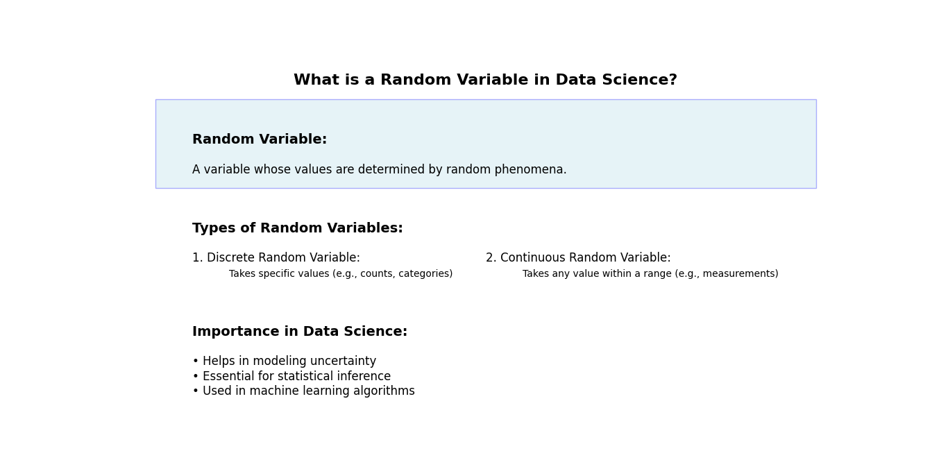
What is a Random Variable?
In data science, a random variable is to represent the results of something random. Its value can change each time you observe the event. For example, when you roll a dice, the result (1 to 6) is a random variable because it’s different every time. Similarly, the number of people visiting a website in an hour is a random variable since it changes each hour.
Key Concepts in Random Variables
To make things clearer, let’s break down a few important terms often used when discussing random variables:
- Stochastic Processes: Processes that involve random variables changing over time, like weather patterns or customer traffic on a website.
- Probability Distributions: The likelihood of each possible value of a random variable. Distributions show patterns of how data behaves.
- Expected Value: The average or central value of a random variable’s possible outcomes, often calculated as a weighted average.
Types of Random Variables: Discrete and Continuous
There are two main types of random variables you’ll encounter in data science:
- Discrete Random Variables: These are variables that take on a countable number of values. An example would be the number of students in a class. There’s no halfway; you either have 20 students, 21 students, and so on.
- Continuous Random Variables: Unlike discrete variables, continuous random variables can take any value within a range. Height, temperature, and weight are classic examples, as these measurements can vary continuously without clear jumps from one value to the next.
Here’s a quick overview of the types of random variables:
| Type | Description | Examples |
|---|---|---|
| Discrete | Countable outcomes, usually integers | Number of website clicks, rolls of a dice |
| Continuous | Any value within a range | Temperature, time, weight |
Examples of Random Variables in Real-World Data Science
Now, let’s look at some real-world applications where random variables show up:
- Customer Purchase Behavior: In e-commerce, the number of purchases by each customer is a random variable. Analyzing this helps predict future sales patterns.
- Weather Forecasting: Temperature on any given day is a continuous random variable. Weather models use random variables to estimate the likelihood of conditions like rain or snow.
- Financial Modeling: Stock prices are treated as random variables to account for fluctuations due to market conditions. Here, we use stochastic processes to model how prices might change over time.
Example Code in Python
Let’s see a quick Python example. This code shows how we might model the number of daily visitors to a website. Each visitor count is a discrete random variable.
import numpy as np

# Simulate daily visitors over 10 days
np.random.seed(0)
daily_visitors = np.random.poisson(lam=100, size=10)

print("Daily visitors over 10 days:", daily_visitors)
In this code, the Poisson distribution is used to simulate daily visitor counts. Here, lam=100 represents an average of 100 visitors per day.
Probability Distributions in Random Variables
Probability distributions are crucial in data science. They show how likely each possible outcome is. Let’s look at a few common ones:
- Binomial Distribution: Used for events with two possible outcomes, like flipping a coin.
- Normal Distribution: Data clusters around an average, like people’s heights.
- Poisson Distribution: Useful for counting events, like the number of cars passing a toll booth.
Why Random Variables Matter in Data Science
Random variables help data scientists manage uncertainty. They let us assign probabilities to unpredictable outcomes, improving decision-making and predictions. Without random variables, analyzing random data would be much harder.
Summary
- Random Variables in data science allow us to manage unpredictable data.
- Discrete Random Variables have set values; Continuous Random Variables take any value within a range.
- Examples include customer behavior, stock predictions, and weather patterns.
By understanding random variables, we can use randomness in data science to reveal patterns and make better decisions. With these tools, you’re ready to start analyzing real-world data.
Understanding Probability Distributions for Data Modeling
Probability distributions are crucial when working with data science. They help you understand how data behaves and allow for accurate predictions. When you look at a random variable in data science, knowing its probability distribution can reveal patterns and provide a clearer picture of what to expect from the data.
Probability distributions might seem complex at first, but understanding them can improve data modeling, which is the foundation of data science and machine learning.
What Are Probability Distributions?
In simple terms, a probability distribution shows how the values of a random variable are spread out or distributed. This helps you understand how likely it is for the variable to take on certain values.
For example, if you roll a fair six-sided die, each outcome (from 1 to 6) has an equal probability. This is a uniform distribution because each number has the same likelihood of appearing.
Key Concepts in Probability Distributions
There are a few main points to keep in mind:
- Random Variables in Data Science: In data science, random variables represent events or outcomes, and probability distributions give structure to their randomness.
- Probability Density Function (PDF): For continuous random variables, the PDF shows the probability of the variable falling within a specific range.
- Probability Mass Function (PMF): For discrete random variables, the PMF gives the probability of each individual outcome.
Here’s a quick breakdown to make it clearer:
| Type | Explanation | Examples |
|---|---|---|
| Probability Density Function (PDF) | Used for continuous random variables | Heights of people, temperatures |
| Probability Mass Function (PMF) | Used for discrete random variables | Number of heads in coin flips |
Must Read
- How to Debug ML Inference Latency and Throughput Issues
- Shadow Deployment and Canary Testing for Machine Learning Models: A Practical Guide
- How to Build an ML Monitoring Dashboard from Scratch (Streamlit Tutorial)
- ML Model Monitoring: How to Detect Data Drift and Model Decay in Production
- Retrain vs Fine-Tune vs Train from Scratch: A Decision Framework for ML Engineers
Types of Probability Distributions
Understanding the Normal Distribution in Data Science
The Normal Distribution, also known as the Gaussian Distribution, is one of the most commonly used probability distributions in data science. This distribution is fundamental to data modeling, statistical analysis, and various machine learning algorithms. Its shape—a bell curve—reflects how data clusters around a central value, with the frequency of values gradually decreasing on either side as they move away from the center.
Key Characteristics of Normal Distribution
The Normal Distribution has distinct characteristics that make it predictable and useful for modeling:
- Mean (μ): This is the average value, and it determines where the center of the bell curve lies.
- Standard Deviation (σ): A measure of the data’s spread around the mean. A smaller standard deviation indicates that the data points are closer to the mean, resulting in a steeper curve. A larger standard deviation spreads the data out, creating a wider, flatter curve.
- Symmetry: The curve is symmetrical, so the probabilities are identical on both sides of the mean.Symmetry: The curve is symmetrical, so the probabilities are identical on both sides of the mean.
These characteristics make the normal distribution very predictable, as around 68% of data points fall within one standard deviation from the mean, 95% fall within two, and 99.7% fall within three. This is often called the 68-95-99.7 rule.
Mathematical Representation: Probability Density Function (PDF)
The Probability Density Function (PDF) gives the probability of different values in a dataset distributed normally. The formula for the normal distribution is:
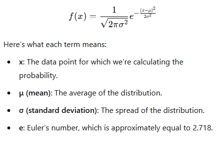
What Does the Formula Do?
This formula tells us how likely it is for a value (x) to occur within a normal distribution defined by μ and σ. It’s especially useful in data modeling when estimating how likely new data points will fit within a distribution.
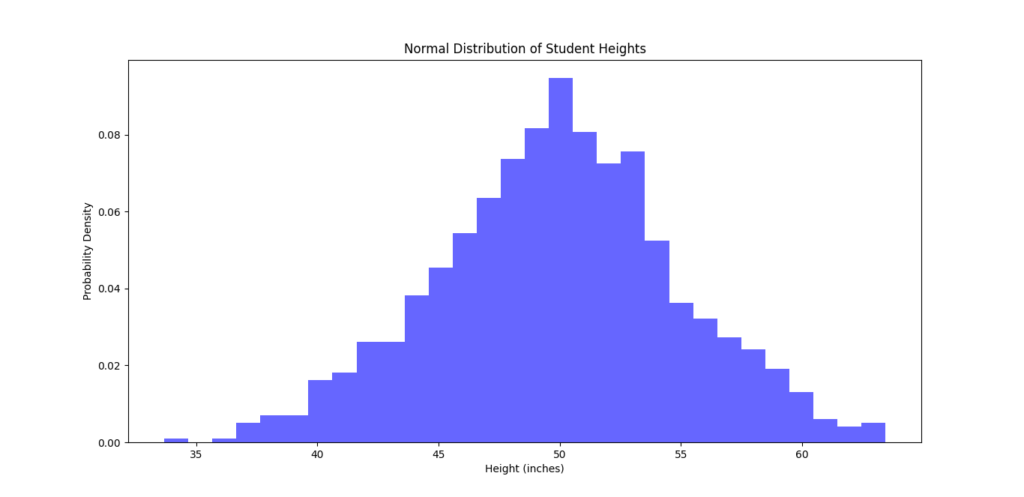
Visual Example: Heights of Students
Let’s say we want to model the heights of students in a class. Generally, most students have a height around a specific average, with fewer students being significantly shorter or taller. This situation naturally follows a normal distribution.
Assume:
- Mean height (μ) = 50 inches
- Standard deviation (σ) = 5 inches
The normal distribution model helps us determine the probability of a student having a specific height. Most students’ heights are likely to be close to the average, typically within one standard deviation (between 45 and 55 inches). Fewer students will have heights much shorter or taller than the average, such as below 40 inches or above 60 inches.
Python Example: Visualizing the Normal Distribution
Using Python, we can generate and plot a normal distribution to visualize this concept.
import numpy as np
import matplotlib.pyplot as plt

# Generate data for a normal distribution
data = np.random.normal(loc=50, scale=5, size=1000)  # Mean=50, StdDev=5

# Plot the normal distribution
plt.hist(data, bins=30, density=True, alpha=0.6, color='b')
plt.title("Normal Distribution of Student Heights")
plt.xlabel("Height (inches)")
plt.ylabel("Probability Density")
plt.show()
In this code:
- We generate 1000 random data points using
np.random.normal(), centered around 50 with a standard deviation of 5. - Then, we plot these values on a histogram to see the bell-shaped curve typical of a normal distribution.
The output shows that most values cluster around the mean (50), with decreasing frequencies as we move away from this center.
When to Use the Normal Distribution
The normal distribution is ideal for data modeling when:
- Data clusters around a mean with relatively equal variation on either side.
- Symmetry is observed in the distribution of values, where data tails off equally in both directions.
Real-Life Use Cases
- Quality Control: In manufacturing, measuring product dimensions can follow a normal distribution where the average dimension is the target, with variations representing acceptable tolerance levels.
- Standardized Testing: Exam scores often follow a normal distribution, where the mean score represents the average student performance, and scores are symmetrically spread around this mean.
- Natural Phenomena: Many biological and social data types, like human weights or blood pressure levels, also follow normal distributions due to natural variability around an average.
Example Problem: Applying Normal Distribution to Calculate Probabilities
Suppose we want to calculate the probability of a randomly chosen student being between 45 and 55 inches tall. We know that for a normal distribution:
- 68% of data falls within 1 standard deviation (μ ± σ).
- 95% of data falls within 2 standard deviations (μ ± 2σ).
- 99.7% of data falls within 3 standard deviations (μ ± 3σ).
So, with μ = 50 and σ = 5:
- 68% of students will likely have heights between 45 (50 – 5) and 55 (50 + 5) inches.
Summary of Key Concepts
- Normal Distribution models data clustering around a central value.
- It has a bell-shaped curve, symmetrical around the mean.
- Use it for data that is evenly spread around an average, like heights, weights, and scores.
This analysis should provide a good foundation for understanding the Normal Distribution and its practical applications in data science. It’s a powerful tool for estimating probabilities and making informed predictions when your data meets the right conditions.
Understanding the Binomial Distribution in Data Science
The Binomial Distribution is a probability distribution used to model scenarios with two possible outcomes in each trial, often labeled as success or failure. This distribution is perfect for analyzing situations where each trial or event has only two outcomes, like a yes-or-no survey response, flipping a coin, or measuring whether a machine part passes or fails quality control.
Let’s break down the key features, mathematical formula, and applications of the Binomial Distribution, along with examples and Python code to help you visualize it.
Key Characteristics of the Binomial Distribution
The binomial distribution has a few defining characteristics:
- n (Number of Trials): This represents how many times the experiment is conducted. For example, in flipping a coin 10 times, n = 10.
- p (Probability of Success): This is the likelihood of achieving the desired outcome in each trial. For example, the probability of flipping heads on a fair coin is p = 0.5.
- Discrete Distribution: Since the possible outcomes are limited (either a success or failure in each trial), the binomial distribution applies to discrete values.
This distribution is commonly used in scenarios where you’re observing a certain number of independent events with a fixed probability of success, each yielding either a success or a failure.
Binomial Distribution Formula
The probability mass function (PMF) for the binomial distribution is as follows:
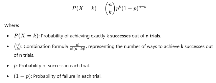
What Does the Formula Mean?
This formula calculates the probability of getting exactly k successes in n independent trials, each with the same probability of success p. This is useful in scenarios like customer churn analysis, where each customer either stays (success) or leaves (failure) within a certain period.
Real-World Example: Coin Flipping
To understand this, let’s apply it to flipping a fair coin.
- Scenario: Flipping a coin 10 times and observing how many times it lands on heads.
- Parameters:
- n = 10 (10 trials)
- p = 0.5 (probability of heads)
- Question: What’s the probability of getting exactly 6 heads in 10 flips?
Using the binomial formula:
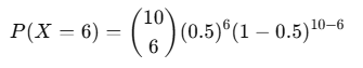
Calculating this would give you the probability of observing exactly 6 heads in 10 coin flips.
Python Example: Visualizing the Binomial Distribution
With Python, we can simulate a binomial distribution to see how likely we are to get a certain number of heads in multiple trials.
import numpy as np
import matplotlib.pyplot as plt

# Simulate a binomial distribution with 10 trials, probability of success = 0.5
binomial_data = np.random.binomial(n=10, p=0.5, size=1000)

# Plot the binomial distribution
plt.hist(binomial_data, bins=10, density=True, alpha=0.7, color='g')
plt.title("Binomial Distribution of Coin Flips")
plt.xlabel("Number of Heads")
plt.ylabel("Probability Density")
plt.show()
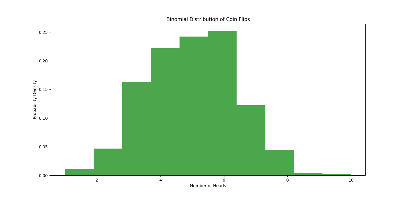
In this example:
np.random.binomial()generates 1000 simulated outcomes of flipping a coin 10 times.- The histogram displays the distribution of heads across these trials, showing us how likely each outcome is, from getting no heads to getting all 10 heads.
The result is a histogram where we can see the most common outcomes (like 5 heads) compared to rarer outcomes (like 0 or 10 heads).
When to Use the Binomial Distribution
The Binomial Distribution is ideal for data analysis when:
- Binary Outcomes: Each trial has only two possible outcomes, like success or failure.
- Fixed Number of Trials (n): The number of trials is set before conducting the experiment.
- Independent Trials: Each trial’s outcome does not affect the others.
- Constant Probability (p): The probability of success is the same for each trial.
Practical Use Cases
- Quality Control: For example, in manufacturing, each product could either pass or fail inspection. The binomial distribution can estimate the probability of producing a certain number of faulty items in a batch.
- Customer Behavior Analysis: In customer retention, where each customer either stays or churns (leaves). Analysts can use the binomial distribution to predict the likelihood of a certain number of customers leaving in a given period.
- Drug Effectiveness: In clinical trials, where a new drug might either work or not for each patient. The binomial distribution can help estimate the success rate of the drug over a set number of patients.
Example Problem: Customer Churn Analysis
Suppose a telecom company wants to model customer churn rates:
- Scenario: Out of 100 customers, each customer has a 10% probability of churning.
- Question: What’s the probability of exactly 15 customers leaving?
Using the binomial formula, you’d set:
- n = 100 (100 customers)
- p = 0.1 (10% probability of churning)
- k = 15 (looking for exactly 15 customers to churn)
The Binomial PMF can give the likelihood of observing exactly 15 churns, which is valuable for predicting financial risk or planning marketing interventions.
Summary of Key Concepts
- Binomial Distribution models events with two outcomes over a set number of trials.
- It requires a fixed number of trials, constant success probability, and independence of trials.
- Use cases include customer churn, quality control, and experimental trials.
Understanding the Binomial Distribution can help you make informed predictions in data science, especially when working with categorical data that fits a binary framework. By knowing when and how to apply this distribution, you can add powerful probability analysis to your data toolkit.
Understanding the Poisson Distribution in Data Science
The Poisson Distribution is a vital probability distribution used in data science to model the number of times an event occurs in a fixed interval of time or space. It is particularly useful when dealing with events that occur randomly and independently at a constant average rate.
Let’s explore the characteristics, mathematical formulation, applications, and practical examples of the Poisson Distribution.
Key Characteristics of the Poisson Distribution
- λ (Lambda): This parameter represents the average rate of occurrence of events in a specified interval. For instance, if a store sees an average of 4 customers per hour, then λ = 4.
- Discrete Distribution: Since the Poisson distribution counts the number of events, the possible outcomes are whole numbers (0, 1, 2, …).
- Independence: Events are considered independent, meaning the occurrence of one event does not influence the occurrence of another.
Poisson Distribution Formula
The probability mass function (PMF) for the Poisson distribution is expressed as follows:
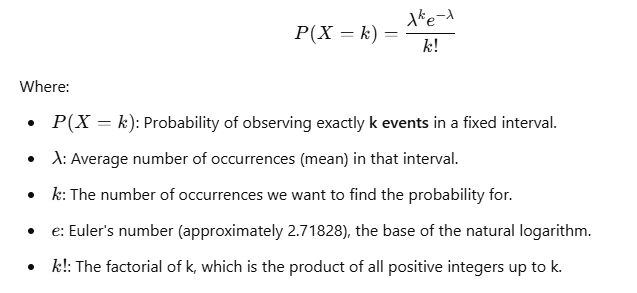
Understanding the Formula
This formula tells us how likely it is to observe exactly k events given that the average occurrence rate is λ. This is useful in various fields like queueing theory, telecommunications, and inventory management.
Real-World Example: Customer Arrivals at a Store
Let’s consider a situation where we want to predict how many customers visit a store in an hour. On average, we know that 4 customers arrive per hour. This kind of scenario can be modeled using the Poisson distribution, which is often used to describe the probability of a given number of events (like customer arrivals) occurring within a fixed time period.
- Scenario: You want to find out the probability of exactly 2 customers arriving in the next hour.
- Parameters:
- λ = 4 (average number of customers arriving per hour)
- k = 2 (the number of customers for which we want to find the probability)
Using the Poisson formula:
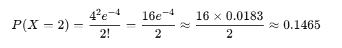
This means there is approximately a 14.65% chance of exactly 2 customers arriving in that hour.
Python Example: Visualizing the Poisson Distribution
Let’s visualize this scenario using Python to see how customer arrivals follow a Poisson distribution.
import numpy as np
import matplotlib.pyplot as plt

# Simulate a Poisson distribution with lambda = 4
poisson_data = np.random.poisson(lam=4, size=1000)

# Plot the Poisson distribution
plt.hist(poisson_data, bins=10, density=True, alpha=0.7, color='orange')
plt.title("Poisson Distribution: Customer Arrivals")
plt.xlabel("Number of Customers")
plt.ylabel("Frequency")
plt.xticks(range(0, 11))
plt.show()
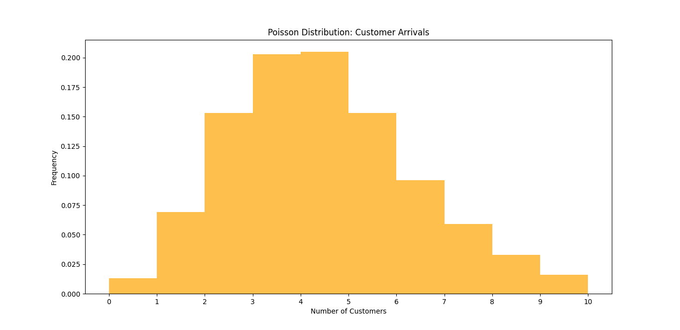
In this code:
- We use
np.random.poisson()to generate 1000 samples from a Poisson distribution with an average of 4 customers. - The histogram displays the distribution of customer arrivals, illustrating how frequently we expect to see different numbers of customers within that hour.
When to Use the Poisson Distribution
The Poisson Distribution is particularly useful in the following scenarios:
- Modeling Rare Events: When you’re interested in counting the occurrence of events that are rare or infrequent within a fixed interval (e.g., the number of earthquakes in a year).
- Queueing Systems: In service industries, like restaurants or banks, to predict customer arrivals or service requests.
- Traffic Analysis: Analyzing the number of calls received by a call center in an hour or the number of requests received by a server in a minute.
- Machine Failures: Estimating how many times a machine might fail in a day or week, which helps in maintenance planning.
Example Problem: Website Traffic Spikes
Suppose a website typically experiences an average of 5 visits per minute. You might want to model the probability of experiencing 3 visits in a single minute.
- Scenario: Find the probability of receiving exactly 3 visits in that minute.
- Parameters:
- λ = 5 (average number of visits)
- k = 3 (the specific number of visits)
Using the Poisson formula:
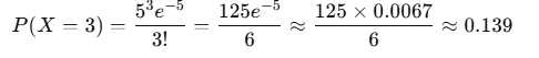
This indicates a 13.9% chance of receiving exactly 3 visits in that minute.
Summary of Key Concepts
- The Poisson Distribution models the number of events in a fixed interval when events happen at a constant rate.
- It is defined by the parameter λ, which represents the average number of occurrences.
- The PMF formula provides the probability of observing a certain number of events.
- Use cases include customer arrivals, website traffic, machine failures, and rare event counts.
Understanding the Poisson Distribution is important for data scientists as it provides powerful insights into the frequency of events within defined intervals. By using this distribution, you can enhance your analyses and decision-making in various applications.
Understanding the Exponential Distribution
The Exponential Distribution is a key concept in probability theory and statistics, particularly useful for modeling the time between events in a Poisson process. It describes the time until a specific event occurs, making it essential in various fields, including engineering, telecommunications, and finance.
Key Characteristics of the Exponential Distribution
- Mean: The mean of the exponential distribution is given by 1\λ, where λ is the rate parameter. This represents the average time between events. For example, if λ=0.5, the average time until the event occurs would be 2 time units.
- Memoryless Property: A unique characteristic of the exponential distribution is its memoryless property, which means the probability of an event occurring in the next interval is independent of how much time has already elapsed. For example, if you’ve already waited for 5 minutes for a bus, the probability of it arriving in the next 2 minutes remains the same as if you had just started waiting.
Probability Density Function (PDF)
The probability density function (PDF) of the exponential distribution is given by:
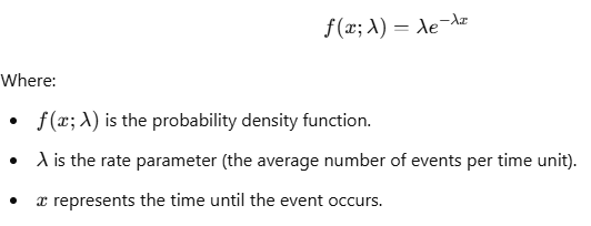
This function indicates how likely it is to observe a certain time xxx until the next event.
Real-World Example: Machine Failure
Consider a factory where a specific machine part has a constant failure rate. Let’s say the average failure rate (λ) is 0.5 failures per hour.
- Scenario: You want to model the time until the part fails.
- Parameters:
- λ = 0.5 (average failure rate)
- The mean time until failure would be 1\λ=2hours.
Using the exponential PDF, we can calculate the probability of the part failing within a certain time frame.
For example, to find the probability of failure within the first hour, we can use the cumulative distribution function (CDF):
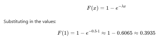
This means there is approximately a 39.35% chance that the machine part will fail within the first hour.
Python Example: Visualizing the Exponential Distribution
Let’s visualize the exponential distribution using Python to better understand how it models the time until an event occurs.
import numpy as np
import matplotlib.pyplot as plt

# Simulate an exponential distribution with lambda = 0.5
exponential_data = np.random.exponential(scale=2, size=1000)  # scale is 1/lambda

# Plot the exponential distribution
plt.hist(exponential_data, bins=30, density=True, alpha=0.6, color='purple')
plt.title("Exponential Distribution: Time until Failure")
plt.xlabel("Time until Failure (hours)")
plt.ylabel("Frequency")
plt.grid(axis='y', alpha=0.75)
plt.show()
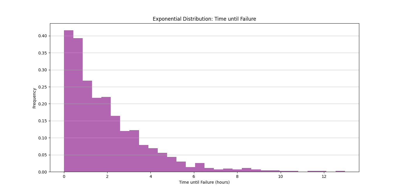
In this code:
- We use
np.random.exponential()to generate 1000 samples from an exponential distribution with a mean of 2 hours (since we setscale=2, which is 1λ). - The histogram displays the distribution of times until the machine part fails, showing how frequently we can expect failures to occur at different time intervals.
When to Use the Exponential Distribution
The Exponential Distribution is particularly useful in scenarios such as:
- Modeling Time Until Events: It is ideal for measuring time intervals between random events, such as:
- Waiting times in queue systems (e.g., how long customers wait in line).
- Time until failure in reliability engineering (e.g., how long machinery operates before breaking down).
- Time between arrivals in a service system (e.g., how long it takes for the next customer to arrive at a restaurant).
- Queueing Theory: In operations research, the exponential distribution is commonly used to model the time between arrivals of customers or calls to a service center.
- Telecommunications: It can model the time until a packet is successfully transmitted over a network or the time between successive events in a system.
Example Problem: Waiting Time in a Queue
Suppose a customer service desk receives calls at an average rate of 2 calls per hour. We can model the time until the next call using the exponential distribution.
- Scenario: Find the probability that the next call will arrive within the next 30 minutes.
- Parameters:
- λ = 2 (average rate of calls)
- Mean time until the next call = 1\λ=0.5 hours or 30 minutes.
Using the CDF:
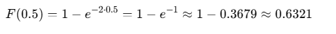
This means there is approximately a 63.21% chance that the next call will arrive within the next 30 minutes.
Summary of Key Concepts
- The Exponential Distribution models the time between events in a Poisson process.
- It is characterized by its mean 1λ\frac{1}{\lambda}λ1 and has a unique memoryless property.
- The PDF provides the probability of observing a certain time until the next event.
- Use cases include measuring time until machine failures, waiting times in queue systems, and inter-arrival times in service processes.
Understanding the Exponential Distribution equips data scientists and analysts with the tools to predict and model time-based phenomena, leading to improved operational efficiencies and decision-making.
Mathematical Properties of Random Variables
What is Expectation (Expected Value) in Data Science?
The expected value of a random variable is like an average, but it takes into account how likely each outcome is. It’s calculated by multiplying each possible outcome by its probability and then adding them up. This gives us an idea of what to expect, on average, from random events. It’s a key concept in predictive modeling and statistical analysis.
The expected value, often denoted as E(X), can be calculated differently depending on whether the random variable is discrete or continuous.
Why is Expected Value Important?
In data science, expected value aids in:
- Estimating averages for predictions.
- Quantifying risk and uncertainty in decisions.
- Evaluating long-term outcomes of probabilistic events.
For instance, if you’re analyzing customer purchases to predict revenue, understanding the mean of random variables can provide insights into average purchase amounts over time.
How to Calculate Expected Value for a Discrete Random Variable
Let’s break down the process for discrete random variables.
Formula
For a discrete random variable X with possible outcomes x1,x2,x3,…,xn, and probabilities p1,p2,p3,…,pn, the expected value E(X) is calculated as:
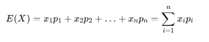
This formula simply states that each outcome xi is weighted by its probability pi, and then all these weighted values are summed up.
Example
Let’s consider a simplified example of flipping a coin three times and observing the number of heads:
| Outcome (Number of Heads) | Probability |
|---|---|
| 0 | 0.125 |
| 1 | 0.375 |
| 2 | 0.375 |
| 3 | 0.125 |
Calculating E(X):
E(X)=(0×0.125)+(1×0.375)+(2×0.375)+(3×0.125)=1.5
So, on average, we expect to see 1.5 heads in three coin flips.
Calculating Expected Value for a Continuous Random Variable
For continuous random variables, things get a bit more complex as we deal with ranges rather than distinct values.
Formula
The expected value for a continuous random variable X with probability density function f(x) is calculated using an integral:
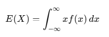
This integration sums up all possible values of x weighted by their probabilities, represented by f(x).
Example: Time Between Customer Arrivals
If customer arrival times in a store are modeled by an exponential distribution with a mean arrival time of 10 minutes, then E(X) would simply be the mean time, which is 10 minutes in this case.
Relation Between Expected Value and Mean
In data science, mean and expected value are often used interchangeably.
- Sample Mean: Calculated from observed data, often used to estimate the expected value.
- Expected Value: Calculated theoretically based on probabilities.
If we had infinite data, the sample mean would exactly equal the expected value. However, with finite data, the sample mean serves as a good approximation.
Practical Example: Calculating Expected Value in Python
Let’s say you want to simulate a dice roll and calculate the expected value for the outcomes.
import numpy as np

# Define possible outcomes and their probabilities
outcomes = np.array([1, 2, 3, 4, 5, 6])
probabilities = np.array([1/6] * 6)

# Calculate expected value
expected_value = np.sum(outcomes * probabilities)
print("Expected Value of a Dice Roll:", expected_value)
Output:
Expected Value of a Dice Roll: 3.5
In this example, each outcome (1 through 6) has an equal probability of 1/6, leading to an expected value of 3.5. So, over many dice rolls, we can expect an average outcome of 3.5.
Visualizing Expected Value
Let’s visualize the expectation to better understand its role:
- Discrete Random Variable: Represented by a bar chart, showing probabilities of each outcome. The expected value can be marked on the x-axis to indicate the center of mass.
- Continuous Random Variable: Illustrated as a curve, with the expected value marked along the x-axis, representing the distribution’s average point.
Key Points to Remember
- Expected Value is foundational in data science for making predictions and decisions.
- Calculating the expected value differs for discrete and continuous random variables.
- In practice, the mean of random variables estimated from data approximates the expected value, providing a basis for interpreting future events.
Variance and Standard Deviation of a Random Variable in Data Science
When exploring random variables in data science, understanding variance and standard deviation becomes important. These statistical measures provide a way to describe data dispersion and variability, revealing how spread out or consistent data points are around an average. These concepts help us interpret data and make informed predictions, whether it’s measuring fluctuations in stock prices, sales, or survey responses.
Why Are Variance and Standard Deviation Important?
In data science, variance and standard deviation help us determine the degree of spread or concentration around the mean of a random variable:
- Variance shows how much the numbers in a data set differ from the average (mean). To find variance, we look at how far each number is from the mean, square those differences (to make sure they’re all positive), and then find the average of those squared differences. This gives us a sense of how spread out the data is, but it’s in squared units, which can be hard to understand.
- Standard deviation is just the square root of variance. Taking the square root puts the measurement back in the same units as the original data (for example, if you’re measuring height in inches, the standard deviation will be in inches too). This makes it easier to interpret and understand how spread out the data is in real terms.
- In short:
- Variance = how much the data is spread out, but in squared units.
- Standard deviation = how much the data is spread out, in the same units as the data itself.
Mathematical Formula for Variance
For a random variable X, with expected (mean) value μ=E(X):
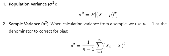
Where:
- X represents each data point.
- μ (population mean) or Xˉ (sample mean) represents the average.
- nnn is the number of observations.
Example of Variance Calculation
Let’s calculate variance with a simple example. Suppose we have data on the number of hours students studied per week:
| Hours Studied (X) | Deviation from Mean (X−μ) | Squared Deviation ((X−μ)2) |
|---|---|---|
| 5 | -3 | 9 |
| 8 | 0 | 0 |
| 10 | 2 | 4 |
| 12 | 4 | 16 |
Steps:
- Calculate the mean μ\muμ: (5+8+10+12)/4=8.75
- Compute each deviation from the mean, square it, and find the average (population variance).
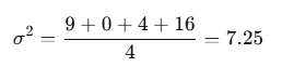
In this case, the variance is 7.25 hours.
What is Standard Deviation?
Standard deviation is the square root of variance, offering an interpretable measure of dispersion in the same unit as the data. The formula is:
σ=square root of σ2
Standard deviation tells us how much variation there is from the mean in a given dataset.
Interpreting Variance and Standard Deviation
These two measures help us answer key questions about a dataset:
- Low Variance and Low Standard Deviation: Data points are close to the mean.
- High Variance and High Standard Deviation: Data points are widely spread around the mean.
In our example, a standard deviation of 2.69 hours suggests that most students studied within a few hours of the average 8.75 hours per week.
Practical Example: Calculating Variance and Standard Deviation in Python
Let’s look at how we can calculate variance and standard deviation in Python.
import numpy as np

# Data: Hours studied per week
hours_studied = np.array([5, 8, 10, 12])

# Calculate population variance and standard deviation
population_variance = np.var(hours_studied)
population_std_dev = np.sqrt(population_variance)

print("Population Variance:", population_variance)
print("Population Standard Deviation:", population_std_dev)
Output:
Population Variance: 7.25
Population Standard Deviation: 2.69
In this example, the output confirms the calculated variance and standard deviation values.
Variance and Standard Deviation in Data Science Applications
- Stock Market Analysis: Variance and standard deviation help evaluate the volatility of stock prices.
- Quality Control: In manufacturing, these measures assess consistency across products.
- Customer Analytics: Understanding customer purchase behaviors by analyzing the variance in spending patterns.
Key Differences: Variance vs. Standard Deviation
| Feature | Variance | Standard Deviation |
|---|---|---|
| Definition | Average squared deviation from mean | Square root of variance |
| Units | Squared units of data | Same units as data |
| Interpretation | More abstract | More interpretable |
| Sensitivity to Outliers | Higher | Less, but still sensitive |
Visualizing Variance and Standard Deviation
To further understand data dispersion, visualizing variance and standard deviation on a graph can be helpful.
In a normal distribution, for instance, 68% of the data falls within one standard deviation from the mean, 95% within two standard deviations, and 99.7% within three standard deviations.
When to Use Variance and Standard Deviation in Data Science
These metrics are valuable when:
- Comparing Consistency: Identify the consistency of different datasets.
- Assessing Risk: Calculate the volatility in financial modeling.
- Quality Assurance: Analyze variations in production.
Covariance and Correlation Between Random Variables in Data Science
In data science, understanding how different variables are related is key to spotting patterns, making predictions, and gaining valuable insights. Two important tools for analyzing these relationships are covariance and correlation.
When we calculate covariance and correlation, we measure how two variables change together. Covariance shows the direction of the relationship—whether the variables move in the same direction or opposite directions. Correlation gives us a clearer picture by showing not only the direction but also the strength of the relationship between the variables.
For example, in fields like finance, biology, and machine learning, correlation is commonly used to identify how variables interact. It helps experts see if two variables tend to rise or fall together (positive correlation) or if one goes up while the other goes down (negative correlation).
Let’s break down both covariance and correlation, their formulas, examples, and when to use each.
What is Covariance?
Covariance tells us how two random variables change in relation to each other. When the covariance is positive, it means that both variables tend to increase or decrease at the same time. On the other hand, if the covariance is negative, it suggests that when one variable increases, the other decreases. It’s like a seesaw, where one side goes up and the other goes down.
Key Characteristics of Covariance:
- Value Range: Covariance values can range widely, making it difficult to interpret the strength of the relationship.
- Direction of Relationship:
- Positive Covariance: Both variables increase or decrease together.
- Negative Covariance: One variable increases while the other decreases.
Formula for Covariance
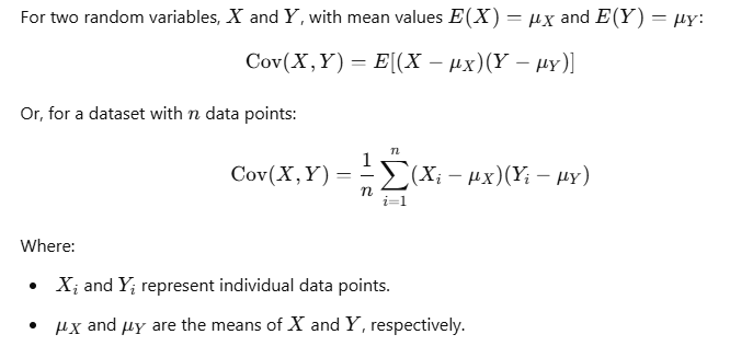
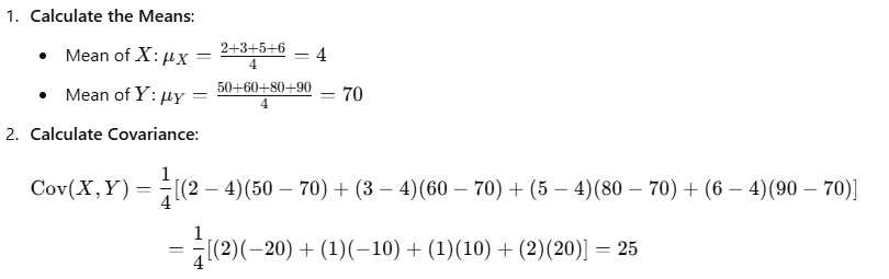
Example of Covariance Calculation
Suppose we want to analyze the relationship between study hours and exam scores among students. Here’s the data:
| Study Hours (X) | Exam Score (Y) |
|---|---|
| 2 | 50 |
| 3 | 60 |
| 5 | 80 |
| 6 | 90 |
What is Correlation?
Correlation takes covariance and puts it on a standardized scale, making it easier to understand the strength and direction of the relationship between two variables. The correlation value ranges from -1 to 1:
- 1 means a perfect positive relationship: as one variable increases, the other always increases in the same way.
- -1 means a perfect negative relationship: as one variable increases, the other always decreases.
- 0 means no linear relationship: the variables don’t show any clear pattern of moving together.
This makes correlation more intuitive because it’s easier to interpret than covariance, and it’s always between -1 and 1.
Formula for Correlation
The correlation coefficient r between two random variables X and Y is:
r=Cov(X,Y)/σX⋅σY
Where:
- σX and σY are the standard deviations of X and Y, respectively.
Example of Correlation Calculation
Using the previous example:
- Calculate Standard Deviations:
- σX (Standard deviation of study hours) = 1.83
- σY (Standard deviation of exam scores) = 17.08
- Calculate Correlation:
r=25/(1.83)(17.08)≈0.81
A correlation of 0.81 suggests a strong positive relationship between study hours and exam scores.
Key Differences: Covariance vs. Correlation
| Feature | Covariance | Correlation |
|---|---|---|
| Purpose | Measures direction of relationship | Measures strength and direction of relationship |
| Scale | Unbounded; depends on data units | Standardized between -1 and 1 |
| Interpretability | Harder to interpret due to scale | Easier to interpret; standardized |
Practical Application of Covariance and Correlation in Data Science
Financial Analysis: In asset returns, a positive covariance between two stocks means that their prices tend to move in the same direction. For example, if one stock’s value rises, the other is likely to rise as well.
Quality Control: In manufacturing, a negative correlation between production speed and defect rate can suggest that as production speed increases, the quality may decrease, leading to more defects.
Customer Analytics: In analyzing customer behavior, a high positive correlation between the time a customer spends on a website and their likelihood to make a purchase could indicate that the longer they browse, the higher their chances of making a purchase.
Using Python to Calculate Covariance and Correlation
Let’s perform both calculations on some sample data to make this more tangible.
import numpy as np

# Data: Hours studied (X) and Exam scores (Y)
hours_studied = np.array([2, 3, 5, 6])
exam_scores = np.array([50, 60, 80, 90])

# Calculate covariance matrix
cov_matrix = np.cov(hours_studied, exam_scores, bias=True)
covariance = cov_matrix[0, 1]

# Calculate correlation coefficient
correlation = np.corrcoef(hours_studied, exam_scores)[0, 1]

print("Covariance:", covariance)
print("Correlation:", correlation)
Output:
Covariance: 25.0
Correlation: 0.81
These calculations confirm our manual results, showing a positive covariance and a strong positive correlation between study hours and exam scores.
Visualizing Correlation
Visualizing correlations can provide clear insights. A scatter plot can illustrate the relationship:
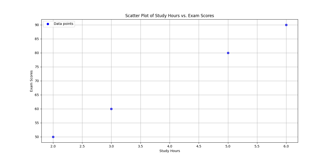
Key Insights on Covariance and Correlation in Data Science
- Use Covariance for Direction: Covariance is helpful to know whether two variables move in the same or opposite direction.
- Use Correlation for Strength and Direction: Correlation standardizes the relationship, allowing easy interpretation of the relationship’s strength.
Practical Tips for Using Covariance and Correlation in Data Science
- When Analyzing Data Relationships:
- Start by calculating correlation for a clear view of the strength of relationships.
- Use covariance if you only need to know the direction without interpreting the strength.
- For Better Visualization:
- Plotting a heatmap of correlations is useful when working with large datasets, making it easy to spot strong positive or negative relationships.
- Avoid Misinterpretation: Correlation does not imply causation. High correlation between two variables does not mean that one causes the other to change.
Applications of Random Variables in Data Science
Random Variables in Predictive Modeling
Predictive modeling is using past data to predict what might happen in the future. For example, predicting sales numbers or stock prices based on historical data.
At the center of this process are random variables. A random variable is something that can change and is often unpredictable. For example, the number of customers that visit a store on any given day is a random variable because it changes every day.
By using random variables in predictive models, we can account for this unpredictability. They help us better understand the uncertainty in our predictions and make more informed guesses about what might happen next.
In simple terms, random variables help us add a level of flexibility and realism to our predictions, allowing data scientists to make more accurate forecasts.
Predictive Models Using Probability
Predictive models rely heavily on the principles of probability to forecast outcomes. Here’s how random variables contribute:
- Modeling Uncertainty: Random variables help us understand and measure the uncertainty in predictions. They show how things might change, giving us a clearer picture of the possible outcomes instead of just one fixed answer.
- Probability Distributions: These distributions (like normal, binomial, or Poisson) tell us how likely different outcomes are. For example, in a normal distribution, most outcomes are close to the average, but some are far away. Knowing this helps us shape better models to predict future events.
- Expected Value Calculation: The expected value is like an average prediction, but it takes into account how likely each outcome is. By calculating the expected value, we can get a sense of the most likely result in a situation, helping us make smarter predictions..
Example: Predicting Sales
Consider a retail company predicting sales for the next quarter. The number of sales can be modeled as a random variable X that follows a Poisson distribution due to the nature of customer arrivals.
The formula for the expected sales can be represented as:E(X)=λ
Where λ is the average number of sales expected in a given time period.
By using historical sales data, the company can estimate λ and use it to forecast future sales, incorporating uncertainty through the random variable model.
Code Snippet: Predicting Sales with Poisson Distribution
Here’s a simple Python code snippet to illustrate this concept:
import numpy as np
import matplotlib.pyplot as plt
from scipy.stats import poisson

# Average sales (lambda)
lambda_sales = 20

# Generate Poisson distribution for sales
sales = np.arange(0, 40)
probabilities = poisson.pmf(sales, lambda_sales)

# Plotting
plt.bar(sales, probabilities, color='blue')
plt.title('Sales Prediction using Poisson Distribution')
plt.xlabel('Number of Sales')
plt.ylabel('Probability')
plt.show()
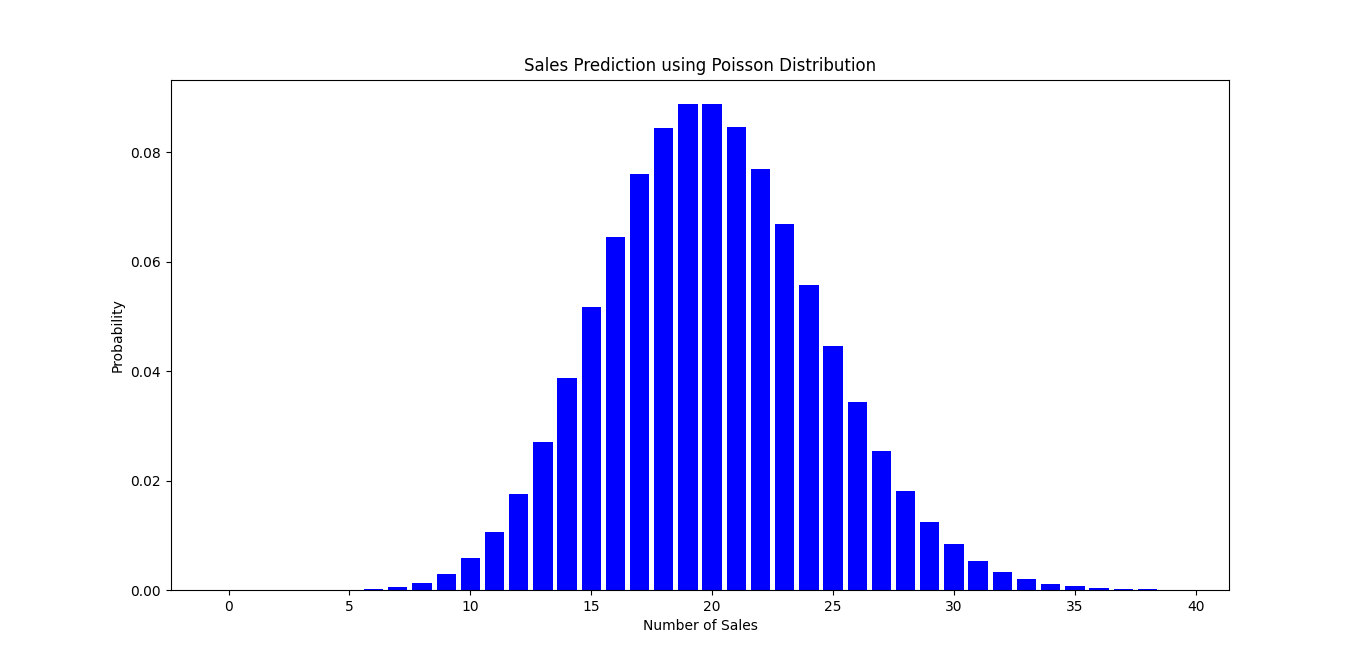
In this plot, the blue bars represent the probability of various sales outcomes. The model effectively uses the random variable X to estimate future sales.
Random Variables in Machine Learning and AI
The Importance of Random Variables in ML
In machine learning and artificial intelligence, random variables are fundamental. They enable models to account for the inherent uncertainty present in real-world data.
- Probabilistic Models: Techniques like Bayesian networks and hidden Markov models use random variables to capture relationships and dependencies between variables, allowing for better predictions and classifications.
Using Probability in Machine Learning
- Feature Representation: Random variables can represent features in a dataset, where each feature may influence the target variable’s outcome.
- Model Evaluation: Probabilistic metrics such as log likelihood are used to evaluate model performance, providing insight into how well a model fits the data.
Example: Classification with Random Variables
In a classification task, suppose we want to predict whether an email is spam or not. Each email can be represented as a set of random variables X1,X2,…,Xn, where each Xi represents a feature (like the presence of certain keywords).
The probability that an email is spam given the features can be modeled using Bayes’ theorem:
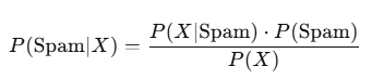
Code Snippet: Spam Detection with Naive Bayes
Here’s a simple implementation using the Naive Bayes classifier in Python:
from sklearn.naive_bayes import GaussianNB
from sklearn.model_selection import train_test_split
from sklearn.metrics import accuracy_score

# Sample dataset (features: X, labels: y)
X = [[1, 1], [1, 0], [0, 1], [0, 0]]  # Example features
y = [1, 0, 0, 0]  # 1 for spam, 0 for not spam

# Splitting the dataset
X_train, X_test, y_train, y_test = train_test_split(X, y, test_size=0.25)

# Model training
model = GaussianNB()
model.fit(X_train, y_train)

# Making predictions
y_pred = model.predict(X_test)

# Accuracy
accuracy = accuracy_score(y_test, y_pred)
print("Accuracy:", accuracy)
In this case, the random variables represent the features of the emails, allowing the model to predict whether they are spam based on their characteristics.
Random Variables in Risk Analysis and Financial Forecasting
The Role of Random Variables in Finance
In risk analysis and financial forecasting, random variables are crucial for assessing and predicting financial risks. They enable analysts to model uncertainties related to investments, market fluctuations, and economic factors.
Using Random Variables for Risk Assessment
- Risk Modeling: Random variables can represent potential losses or gains in various scenarios, helping assess the likelihood of financial outcomes.
- Value at Risk (VaR): This statistical measure estimates the potential loss in value of a portfolio with a given confidence level, utilizing random variables to model returns.
Example: Portfolio Risk Assessment
Consider a portfolio consisting of two assets, A and B. The returns can be modeled as random variables RA and RB.
To calculate the expected portfolio return, we can use:
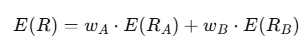
Code Snippet: Portfolio Return Calculation
Here’s a code snippet to calculate the expected return of a simple portfolio:
# Expected returns and weights
returns_A = 0.08  # Expected return for asset A
returns_B = 0.06  # Expected return for asset B
weights = [0.6, 0.4]  # Weights for A and B

# Calculating expected portfolio return
expected_return = weights[0] * returns_A + weights[1] * returns_B
print("Expected Portfolio Return:", expected_return)
In this example, the expected return of the portfolio can be calculated using the assigned weights and the expected returns of each asset.
Latest Advancements in Random Variables for Data Science
In the fast-moving world of data science, new technologies are changing the way we understand and model probability and random variables. Innovations like Generative Adversarial Networks (GANs), Bayesian inference, and even the possibilities of quantum computing are revolutionizing how we approach uncertainty in data. These advancements don’t just improve how we model randomness—they also open up new ways to generate realistic data and make predictions.
This article will dive into these exciting developments, highlighting how random variables continue to play a key role in shaping data science techniques and applications. By exploring these cutting-edge methods, we can better understand the powerful tools available for predicting, analyzing, and generating data.
Generative Adversarial Networks (GANs) and Random Variables
Understanding GANs
Generative Adversarial Networks (GANs) are a revolutionary approach to generative modeling. They consist of two neural networks: a generator and a discriminator, which work against each other in a game-like scenario.
- Generator: This network creates new data samples.
- Discriminator: This network evaluates whether the samples are real (from the training data) or fake (from the generator).
The Role of Random Variables in GANs
Random variables are integral to the functioning of GANs. Here’s how they contribute:
- Input to the Generator: The generator begins with random noise, represented as a random variable Z. This noise is sampled from a simple distribution (e.g., Gaussian) to create diverse outputs.
- Output Distribution: The generator’s goal is to model the distribution of the training data X. It learns to transform the random variable Z into a random variable X′ that closely resembles X.
- Loss Function: The discriminator’s feedback guides the generator through its loss function, which often incorporates probabilities associated with the outputs, illustrating the connection between random variables and generative modeling.
Example: Image Generation
To illustrate, consider a GAN trained to generate images of cats. The generator receives random noise as input:Z∼N(0,1)
Code Snippet: Simple GAN Implementation
Here’s a basic Python snippet showcasing a GAN framework using TensorFlow:
The generator then transforms this input into a realistic cat image. Over time, through adversarial training, it learns to produce images that are statistically similar to actual cat images from the training dataset.
Code Snippet: Simple GAN Implementation
Here’s a basic Python snippet showcasing a GAN framework using TensorFlow:
import numpy as np
import tensorflow as tf
from tensorflow.keras import layers

# Generator Model
def build_generator():
    model = tf.keras.Sequential()
    model.add(layers.Dense(128, activation='relu', input_shape=(100,)))
    model.add(layers.Dense(784, activation='sigmoid'))
    return model

# Discriminator Model
def build_discriminator():
    model = tf.keras.Sequential()
    model.add(layers.Dense(128, activation='relu', input_shape=(784,)))
    model.add(layers.Dense(1, activation='sigmoid'))
    return model

# Instantiate models
generator = build_generator()
discriminator = build_discriminator()

# Random noise input
random_noise = np.random.normal(0, 1, (1, 100))
generated_image = generator.predict(random_noise)
In this snippet, a random variable representing noise is transformed into an image, showcasing the direct involvement of random variables in the GAN framework.
Bayesian Inference and Probabilistic Programming
Understanding Bayesian Inference
Bayesian inference is a statistical method that helps us update the probability of a hypothesis as we gather more evidence or information. Instead of just using a single estimate, like traditional methods do, Bayesian inference uses random variables to account for uncertainty. This approach allows for more flexible and dynamic predictions because it continuously updates its understanding based on new data. Essentially, Bayesian methods help us make better decisions by improving our estimates as we learn more over time.
Advancements in Probabilistic Programming
Probabilistic programming languages, like PyMC3 and TensorFlow Probability, enable data scientists to model complex probabilistic models in an intuitive manner. These languages allow for:
- Hierarchical Modeling: Building models with multiple levels of uncertainty.
- Flexible Priors: Assigning prior distributions to random variables based on previous knowledge.
Example: Disease Prediction
Suppose we want to predict the probability of a patient having a disease based on certain symptoms. The hypothesis can be modeled as a random variable HHH with prior probability P(H). As new symptoms are observed, the posterior probability is updated using Bayes’ theorem:
P(H∣E)=P(E)/P(E∣H)⋅P(H)
Where:
- E is the evidence (observed symptoms).
- P(H | E) is the updated probability of the hypothesis given the evidence.
Code Snippet: Bayesian Inference with PyMC3
Here’s a basic implementation of Bayesian inference:
import pymc3 as pm
import numpy as np

# Simulated data
data = np.random.binomial(1, 0.7, size=100)  # 70% success rate

# Bayesian Model
with pm.Model() as model:
    p = pm.Beta('p', alpha=1, beta=1)  # Prior distribution
    observations = pm.Bernoulli('obs', p=p, observed=data)
    trace = pm.sample(1000)

# Posterior distribution
pm.plot_posterior(trace)
In this example, a Beta distribution is used as a prior for the success probability p, showcasing how random variables are employed in Bayesian inference.
Impact of Quantum Computing on Random Variables
Quantum Computing: A New Frontier
Quantum computing represents a paradigm shift in computing, using the principles of quantum mechanics to process information. Its impact on data science and probability is profound.
Future of Probability in Data Science
Quantum computing can enhance probabilistic modeling in the following ways:
- Superposition and Entanglement: These principles allow for the representation of multiple states simultaneously, which can lead to faster computations for complex probabilistic models.
- Quantum Algorithms: Algorithms like Grover’s and Shor’s can potentially revolutionize how we calculate probabilities and optimize random variables in data science.
Example: Quantum Sampling
Imagine a quantum algorithm designed to sample from a complex probability distribution. Such a capability could dramatically speed up tasks such as Monte Carlo simulations, commonly used for risk analysis and financial forecasting.
Advancements in Probabilistic Data Science
With quantum computing on the horizon, researchers are exploring new algorithms and techniques that integrate random variables more effectively. The potential for advancements in probabilistic data science is immense, paving the way for more accurate models and insights.
Common Challenges in Understanding and Applying Random Variables
Understanding random variables is crucial in data science, but it comes with its own set of challenges. Misconceptions and common pitfalls can hinder your ability to apply these concepts effectively. This article will explore these challenges and provide troubleshooting tips to help data scientists navigate the complexities of probability.
Misconceptions and Pitfalls with Random Variables
Common Errors in Probability
In the realm of data science, numerous misconceptions surround random variables and probability. Some common errors include:
- Confusing Random Variables with Outcomes:
- Misconception: A random variable is often mistaken for a specific outcome.
- Clarification: A random variable is a function that assigns numerical values to outcomes in a sample space. For instance, if X represents the outcome of rolling a die, X can take on values from 1 to 6, while the specific result of a single roll (say, 4) is just an outcome.
- Ignoring Distribution Types:
- Misconception: It is easy to assume all random variables follow the same distribution.
- Clarification: Different types of random variables (discrete vs. continuous) require different handling and understanding. For example, a discrete random variable, like the number of heads in a series of coin flips, can be modeled using a binomial distribution, while a continuous random variable, like the height of individuals, follows a normal distribution.
- Neglecting to Consider Independence:
- Misconception: Many assume random variables are independent by default.
- Clarification: Independence must be explicitly defined. For instance, in a game of dice, the result of one die does not affect another, but this must be stated; otherwise, correlations can lead to incorrect conclusions.
Avoiding Mistakes in Probability
To avoid these common pitfalls, consider the following tips:
- Always Define Random Variables Clearly: Make sure to specify whether a variable is discrete or continuous and what its possible values are.
- Understand the Underlying Distributions: Familiarize yourself with different types of probability distributions (e.g., normal, binomial, Poisson) and their characteristics.
- Examine Relationships Between Variables: Use statistical tests to check for independence or correlation. This is particularly important when developing models that involve multiple random variables.
Troubleshooting and Tips for Data Scientists
Troubleshooting in Data Science
Even experienced data scientists can encounter challenges when working with random variables and probability. Here are some troubleshooting tips to consider:
- Double-Check Data Sources:
- Ensure the data used for analysis is clean and well-understood. Misinterpreted or incomplete data can lead to incorrect modeling of random variables.
- Validate Model Assumptions:
- Always validate the assumptions of the model being used. For example, check if the data truly follows a normal distribution if you’re using techniques that require this assumption.
- Use Visualizations:
- Visual aids can clarify relationships and distributions. Graphs and plots help to visually represent data and identify patterns or anomalies that may indicate errors.
Tips for Learning Probability in Data Science
To strengthen your understanding of probability and random variables, try these practical tips:
- Practice with Real-World Data: Engaging with datasets from real-world scenarios can solidify your understanding of how random variables operate in practice.
- Utilize Online Resources and Courses: Many platforms offer comprehensive courses on probability and statistics tailored to data science.
- Join Community Forums: Engaging with a community of learners can provide support, insights, and answers to common questions or confusions.
Avoiding Common Data Science Errors
Lastly, to prevent common errors, consider these strategies:
- Conduct Peer Reviews: Collaborating with others and sharing your findings can provide fresh perspectives and highlight potential mistakes.
- Stay Updated on Best Practices: Data science is a rapidly evolving field. Keep learning about new techniques and methodologies to enhance your skill set.
- Document Your Work: Keep thorough records of your assumptions, models, and findings. This practice aids in tracing back steps and identifying where things may have gone wrong.
Conclusion: Mastering Random Variables for Data Science Success
In this exploration of random variables, it has become evident that their understanding is vital for anyone pursuing a career in data science. As we’ve discussed, random variables serve as the building blocks for many statistical models and are essential in accurately interpreting data. They provide a framework for quantifying uncertainty and variability, which are inherent in most datasets.
Recap of the Importance of Random Variables in Data Science
Random variables are crucial because they enable data scientists to:
- Quantify Uncertainty: In a world filled with unpredictable events, random variables allow for a structured approach to measure and manage uncertainty. By assigning numerical values to outcomes, insights can be drawn that help in decision-making.
- Model Relationships: They help illustrate how different variables interact with each other. This is especially important in machine learning, where understanding the relationship between input and output variables is fundamental to developing accurate predictive models.
- Apply Advanced Techniques: Many advanced data science methods, such as Bayesian inference and Generative Adversarial Networks (GANs), rely on random variables. Mastering these concepts lays a solid foundation for exploring more sophisticated algorithms and techniques.
Encouragement to Explore More Advanced Topics
As you continue your journey in data science, consider this a stepping stone to delve into advanced data science topics. The realm of probability is vast, offering opportunities to learn about:
Bayesian Statistics: Understanding how to update probabilities as new information becomes available can transform your approach to data analysis.
Markov Chains and Processes: These concepts are vital for modeling random processes where future states depend on the current state, commonly used in AI and machine learning.
Monte Carlo Simulations: A powerful technique for understanding the impact of risk and uncertainty in prediction and forecasting models.
Path to Mastery in Data Science
The journey to mastering random variables is an essential part of your path to proficiency in data science. Recognizing their importance in probability will enhance your analytical skills and enable you to tackle complex problems with confidence.
Remember, the world of data science is ever-evolving, and continuous learning is key to staying ahead. Embrace the challenges, explore advanced topics, and leverage the power of probability in your machine learning projects. This commitment to growth will undoubtedly set you on the path to success in your data science career.
So, take the next step. Explore, practice, and continue building on the solid foundation of random variables in your quest to become a master in the field of data science!
External Resources
“Probability and Random Variables”
Author: David Williams
This foundational paper offers an overview of probability theory and random variables, discussing their significance in various fields, including data science.
“A Survey of Random Variable Modeling Techniques”
Authors: Various
This survey explores different modeling techniques using random variables in data science, focusing on their applications and implications in predictive modeling.
Link to Survey
FAQs
What is a random variable?
A random variable is a numerical outcome of a random process. It assigns a numerical value to each possible outcome of an experiment, allowing statisticians and data scientists to analyze and model uncertain events quantitatively. Random variables can be classified as either discrete (taking specific values) or continuous (taking any value within a range).
Why are random variables important in data science?
Random variables are crucial in data science because they enable the modeling of uncertainty and variability in data. By using random variables, data scientists can analyze patterns, make predictions, and evaluate risks in various applications, such as predictive modeling, machine learning, and risk analysis.
How are random variables used in predictive modeling?
In predictive modeling, random variables represent the uncertain outcomes that models aim to predict. For instance, when building a regression model, the response variable is often a random variable influenced by various predictors. By understanding the distribution and properties of these random variables, data scientists can make more accurate predictions and assess the model’s reliability.
Can you give an example of a random variable in a real-world scenario?
Certainly! Consider the time it takes for a customer to complete a purchase on an e-commerce site. This time can be modeled as a random variable since it can vary significantly from one customer to another due to factors like browsing speed and product interest. Analyzing this random variable can help the company optimize the user experience and improve sales strategies.
")


Leave a Reply