Advanced Linear Algebra for Data Science: A Complete Guide
Introduction
Building on part one, this section dives into advanced Linear Algebra for Data Science, which are crucial for creating powerful algorithms. Techniques like Singular Value Decomposition (SVD) and matrix factorization play a key role in systems such as recommendation engines and Latent Semantic Analysis (LSA) for natural language processing (NLP). These tools allow data scientists to simplify massive datasets and uncover hidden patterns and trends.
We’ll also introduce tensors, which extend the concept of matrices. Tensors are fundamental in deep learning models. Modern frameworks like TensorFlow and PyTorch rely heavily on tensor operations to train neural networks efficiently.
Lastly, we’ll touch on quantum linear algebra, an emerging field with the potential to revolutionize matrix operations in the future.
This guide will equip you with the insights and skills to understand and apply these advanced techniques in your projects.
Advanced Linear Algebra Concepts for Machine Learning
Tensors: Expanding Beyond Matrices
What are Tensors in Machine Learning?
Tensors are multi-dimensional arrays that generalize the concept of matrices. While matrices are limited to two dimensions (rows and columns), tensors can have three or more dimensions. This flexibility makes tensors important in deep learning, as they can represent complex data structures like images, which are 3D arrays (height, width, and color channels), or sequences of text and audio.
Key Features of Tensors:
- Multi-Dimensional: Tensors can represent data in any number of dimensions. For example:
- A 1D tensor is a simple array of numbers.
- A 2D tensor is a matrix.
- A 3D tensor might represent a color image, with dimensions for height, width, and color channels.
- Data Representation: Tensors can hold various types of data, making them highly useful in different machine learning contexts.
How Tensors are Used in Deep Learning
Tensors play a critical role in deep learning frameworks like TensorFlow and PyTorch. These frameworks utilize tensor operations to train neural networks efficiently.
Tensor Operations:
In deep learning, tensor operations include addition, multiplication, and reshaping. Here’s a brief overview of these operations:
- Addition: This operation combines two tensors of the same shape. For example, if you have two matrices (2D tensors) of shape 2×2:

Example of Using Tensors in a Neural Network
Let’s look at a simple example of how tensors are used in a deep learning model. We will create a basic neural network using TensorFlow:
import tensorflow as tf

# Create a simple dataset
data = tf.constant([[1.0, 2.0], [3.0, 4.0]], dtype=tf.float32)  # 2D tensor
labels = tf.constant([[0.0], [1.0]], dtype=tf.float32)  # 2D tensor

# Define a simple model
model = tf.keras.Sequential([
    tf.keras.layers.Dense(2, activation='relu', input_shape=(2,)),
    tf.keras.layers.Dense(1, activation='sigmoid')
])

# Compile the model
model.compile(optimizer='adam', loss='binary_crossentropy', metrics=['accuracy'])

# Train the model
model.fit(data, labels, epochs=5)
In this code:
- A 2D tensor
datais created, which serves as the input for our model. - The model is defined using Keras, which is a high-level API for building neural networks in TensorFlow.
- The model is trained using the
fitmethod, which processes the input tensor and learns from the associated labels.
The Importance of Tensors in Deep Learning Frameworks
Tensors are like supercharged containers for data. If you’ve worked with lists or tables, you can think of tensors as the next level. For example:
- A list is one-dimensional (like a single row of numbers).
- A table (or matrix) is two-dimensional (rows and columns).
- A tensor can have many dimensions (think of it like stacking multiple tables).
Why Are Tensors Important in Machine Learning?
- Efficiency:
- Tensors let computers handle huge amounts of data at once.
- This means faster training for machine learning models, especially when working with lots of images or text.
- Flexibility:
- Tensors can hold all sorts of data:
- For images: They store height, width, and color channels.
- For text: They represent words as numbers.
- For audio: They handle time and frequency data.
- Tensors can hold all sorts of data:
- Speed (GPU Acceleration):
- Tensors work well with GPUs (special computer chips for heavy calculations).
- This makes them perfect for speeding up tasks like training a neural network.
In short, tensors help make machine learning faster, more efficient, and capable of handling all kinds of data!
Matrix Factorization Techniques in Recommender Systems
Non-Negative Matrix Factorization (NMF)
Matrix factorization is a useful method in recommendation systems. One popular type is Non-Negative Matrix Factorization (NMF). NMF is great at predicting what users might like. It works well because it breaks down large data into smaller, meaningful parts.
In this section, we will explain NMF in simple terms. We’ll also look at how it is used in recommendation systems. Plus, we’ll see how it uses ideas from linear algebra.
What is Non-Negative Matrix Factorization?
NMF is a matrix factorization technique that breaks down a large matrix into two smaller matrices. All elements in these matrices are constrained to be non-negative. This property is essential because it aligns well with many real-world data scenarios, such as user ratings for movies or products, where negative values do not make sense.
Mathematical Representation
Let’s say we have a matrix R representing user preferences. This matrix has rows for users and columns for items (like movies). NMF aims to approximate R by two matrices W and H:
R≈W×H
- W (User features): This matrix captures the latent factors associated with users.
- H (Item features): This matrix captures the latent factors associated with items.
Both W and H have non-negative entries.
How NMF Works in Recommendation Systems
NMF can help recommend items by discovering hidden patterns in user preferences. Here’s how it typically works:
- Data Preparation: The user-item interaction data is collected and stored in a non-negative matrix R. This matrix can represent ratings given by users to items, with missing values for unrated items.
- Factorization Process: The NMF algorithm decomposes the matrix R into W and H. The factorization identifies underlying features that explain the observed ratings.
- Prediction: Once W and H are obtained, the predicted rating for a user u on an item i can be computed as follows:

Example of NMF in Action
Let’s consider a simplified example. Imagine we have a user-item rating matrix:
| User\Item | Movie A | Movie B | Movie C |
|---|---|---|---|
| User 1 | 4 | 0 | 3 |
| User 2 | 0 | 2 | 0 |
| User 3 | 5 | 1 | 0 |
In this example, the numbers represent user ratings, with 0 indicating that the user did not rate the item.
Using NMF, we can factor this matrix into two matrices W and H. The resulting matrices might look something like this:
Matrix W (User Features):
| User | Feature 1 | Feature 2 |
|---|---|---|
| User 1 | 0.8 | 0.6 |
| User 2 | 0.1 | 0.9 |
| User 3 | 0.9 | 0.4 |
Matrix H (Item Features):
| Item | Feature 1 | Feature 2 |
|---|---|---|
| Movie A | 0.7 | 0.2 |
| Movie B | 0.1 | 0.8 |
| Movie C | 0.5 | 0.6 |
Using these matrices, predictions can be made. For instance, to predict User 2’s rating for Movie A, the calculation would look like this:

Advantages of NMF in Recommender Systems
- Interpretability: The non-negativity constraint makes the results easier to interpret. Each latent feature can represent a specific aspect of user or item characteristics.
- Efficiency: NMF can handle large datasets effectively, making it suitable for real-world applications.
- Scalability: It scales well with the number of users and items, allowing for the implementation of recommendation systems in various domains.
Must Read
- How to Diagnose Overfitting in Machine Learning — 9 Proven Tools
- PyTorch Debugging Checklist: A Systematic Framework to Fix Models That Won’t Learn
- Why sorted() Is Safer Than list.sort() in Production Python Systems
- Monotonic Sequence in Python: 7 Practical Methods With Edge Cases, Interview Tips, and Performance Analysis
- How to Check if Dictionary Values Are Sorted in Python
Linear Algebra in Machine Learning Algorithms
Linear Regression and Matrices
How Linear Regression Uses Matrices
Linear regression is a basic method in statistics and machine learning. It shows how different variables are connected. This method predicts an output variable y using one or more input variables (features) X.
By using matrices, the calculations become faster and easier to understand. This makes linear regression both powerful and simple to use.
Understanding Linear Regression
In linear regression, we express the relationship between the dependent variable (the output) and independent variables (the inputs) as:
y=Xβ+ϵ
Where:
- y is the vector of predicted values.
- X is the matrix of input features.
- β is the vector of coefficients (parameters).
- ϵ is the error term.
Matrix Representation
Let’s break down the parts of linear regression:
- Input Features (Matrix X):
- Each row of X represents a different observation.Each column represents a different feature.For example, consider a dataset of houses with three features: size, age, and location. The matrix might look like this:
| Size (sq ft) | Age (years) | Location (encoded) |
|---|---|---|
| 1500 | 5 | 1 |
| 2000 | 10 | 2 |
| 1800 | 8 | 1 |
| 2200 | 15 | 3 |
In matrix form, this is:
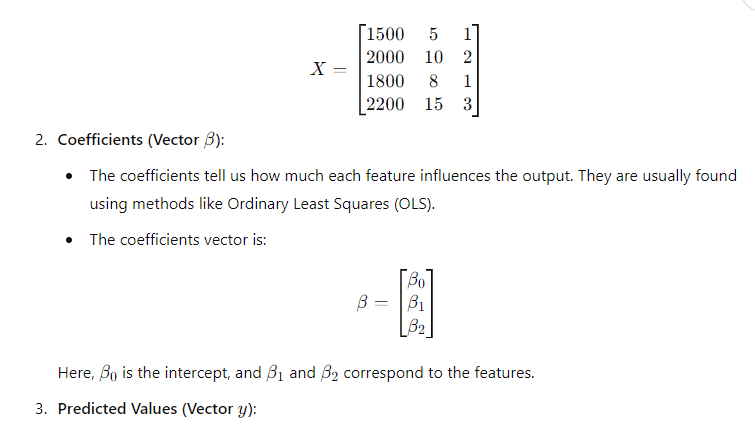
The predicted values for each observation can be calculated with matrix multiplication. We can rewrite our equation as:
y=Xβ
Example of Matrix Multiplication in Linear Regression
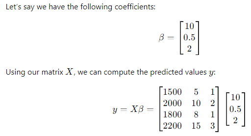
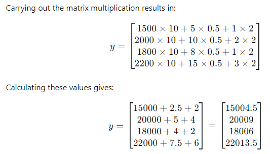
Let’s say we have the following coefficients:
Advantages of Using Matrices in Linear Regression
Using matrices in linear regression has several benefits:
- Efficiency: Matrix operations are faster than traditional methods. This is especially true for large datasets.
- Scalability: Linear regression can easily include more features and observations. Adding data requires only simple changes to the matrix.
- Simplicity: Matrix notation simplifies complex relationships between variables.
Neural Networks and Linear Algebra
Role of Matrices and Vectors in Neural Networks
Neural networks, the building blocks of deep learning, rely heavily on linear algebra to function. At the heart of this are matrices and vectors. These two concepts allow neural networks to process information, learn from data, and make predictions. In this article, we’ll break down how weight matrices and input vectors work together to propagate information both forward and backward in a neural network.
Forward Propagation: How Matrices Move Data Through Neural Networks
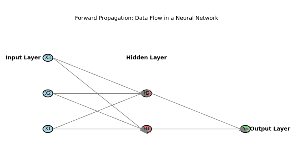
In simple terms, forward propagation refers to the process of sending input data through the network to produce an output. Here, the use of matrices and vectors is essential. When you feed data into a neural network, this data is represented as a vector. For instance, imagine you’re using a network to recognize images. If each image is 28×28 pixels, the input vector will have 784 elements (one for each pixel).
- Input Vector (X): This is the vector that holds the features or data points. Each element corresponds to a specific feature of your input.
- Weight Matrix (W): The weight matrix contains the weights that define how strongly each input feature is connected to each neuron in the next layer.
The forward propagation at each layer is calculated by multiplying the input vector by the weight matrix, followed by adding a bias vector and applying an activation function.
Z=XW+b
Where:
- Z is the result after matrix multiplication (before activation).
- X is the input vector.
- W is the weight matrix.
- b is the bias.
After matrix multiplication, the output is passed through an activation function (like ReLU or sigmoid) to introduce non-linearity:A=activation(Z)
Example of Forward Propagation
Let’s break it down with an example. Imagine we have a simple neural network layer with 3 inputs and 2 neurons. The input vector X could be:
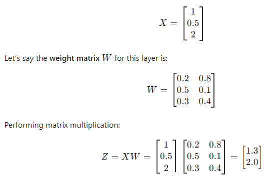
Now, you would add the bias and apply an activation function to produce the final output for this layer.
Backpropagation: Using Matrices to Learn from Errors
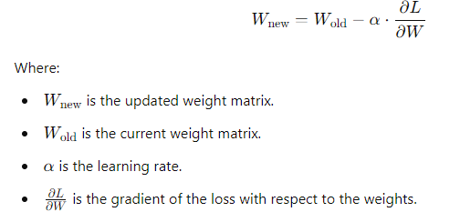
Backpropagation is the process neural networks use to learn by adjusting the weights in the network. This is where matrix operations become even more critical. When the network makes a prediction, errors (or loss) are calculated by comparing the predicted output with the actual target.
Backpropagation uses matrix derivatives (gradients) to adjust the weights in the network. Essentially, it works by moving backward through the network, updating weights at each layer to reduce the error in the next forward pass.
In matrix form, this involves:
- Calculating the gradient of the loss with respect to the weights using the chain rule.
- Multiplying these gradients by a learning rate to determine how much the weights should be updated.
Here’s a simplified equation for weight update:
How Linear Algebra Powers Neural Networks
- Matrix Multiplication: Allows the network to process input data in bulk, propagating information through multiple layers at once.
- Dot Products: Between input vectors and weight matrices determine how inputs get transformed as they move through the network.
- Gradient Descent: Updates weights by calculating derivatives (gradients), using matrix operations to ensure the network improves with each iteration.
Code Example: Forward Propagation in Python (with NumPy)
To see this in action, here’s a simple code snippet that demonstrates forward propagation using NumPy:
import numpy as np

# Input vector (X)
X = np.array([1, 0.5, 2])

# Weight matrix (W)
W = np.array([[0.2, 0.8],
              [0.5, 0.1],
              [0.3, 0.4]])

# Bias vector (b)
b = np.array([0.1, 0.2])

# Perform matrix multiplication and add bias
Z = np.dot(X, W) + b

# Apply activation function (ReLU)
A = np.maximum(0, Z)  # ReLU

print(A)
This example demonstrates how input vectors, weight matrices, and bias terms work together to perform forward propagation in a simple neural network.
Latest Advancements in Linear Algebra for Data Science
Advances in Matrix Factorization Techniques for Big Data
Matrix factorization has always been a powerful tool for machine learning, especially in fields like recommendation systems and data compression. However, the rise of big data has introduced new challenges. Traditional matrix factorization techniques were designed for smaller datasets, and they often struggle to handle the sheer volume and complexity of today’s large-scale datasets. But thanks to recent research and algorithmic developments, matrix factorization has evolved to meet these demands.
In this article, we’ll explore these advances in matrix factorization for big data. We’ll break down the latest research, and algorithms, and explain the underlying concepts with real-world applications. This content is particularly important for learners diving into linear algebra for data science, as it plays a crucial role in managing massive datasets efficiently.
What is Matrix Factorization?
Matrix factorization involves breaking down a large matrix into smaller, more manageable matrices. It’s widely used in fields like:
- Recommendation systems (e.g., Netflix and Amazon)
- Dimensionality reduction (to simplify data)
- Collaborative filtering
For example, in recommendation systems, matrix factorization helps predict a user’s preferences by analyzing relationships between users and items based on previous interactions.
Challenges with Big Data
When working with small datasets, matrix factorization can be done relatively easily using traditional methods like Singular Value Decomposition (SVD) or Non-Negative Matrix Factorization (NMF). But with big data, the situation becomes more complex. Big data brings challenges like:
- High dimensionality: The number of features or attributes can be overwhelming.
- Sparsity: Many matrices in large datasets are sparse, meaning they contain a lot of zeroes.
- Scalability: Traditional methods can’t scale effectively with the volume of data.
These challenges have driven researchers to create new matrix factorization algorithms that are tailored to handle large-scale datasets.
Advances in Matrix Factorization Techniques
1. Stochastic Gradient Descent (SGD)
One of the most widely adopted algorithms for matrix factorization in big data is Stochastic Gradient Descent (SGD). Instead of factoring the entire matrix at once, SGD focuses on small chunks of the data, iteratively adjusting the factorized matrices.
Advantages of SGD:
- Efficiency: It can handle extremely large datasets by breaking down the optimization process into smaller, manageable parts.
- Scalability: Works well with parallel computing, making it ideal for big data.
Example: Let’s consider a matrix RRR that represents user ratings of movies. Instead of processing the entire matrix at once, SGD picks random elements from the matrix and updates the factorized matrices accordingly. This way, the algorithm works in small steps, making it much faster for large datasets.
2. Alternating Least Squares (ALS)
Alternating Least Squares (ALS) is another matrix factorization method optimized for big data. ALS operates by alternating between fixing one matrix while solving for the other. It works iteratively, minimizing the error by focusing on one set of factors at a time.
Advantages of ALS:
- Parallelizable: Since ALS breaks down the factorization into smaller sub-problems, it can be distributed across multiple processors, speeding up the computation.
- Effective for sparse matrices: Many big data applications, such as recommendation systems, have sparse data. ALS handles sparse matrices efficiently.
ALS in Action: In a recommendation system, ALS first holds the user feature matrix constant and solves for the item matrix. Then, it does the reverse, holding the item matrix constant and solving for the user matrix. This alternating process continues until the error is minimized.
3. Non-Negative Matrix Factorization (NMF) for Big Data
NMF is a technique that breaks a matrix down into two smaller matrices where all elements are non-negative. This method is especially useful in fields like topic modeling and image analysis. Recent research has extended NMF to handle large-scale datasets more efficiently.
Improvements in NMF for Big Data:
- Sparse NMF: Handles sparse matrices effectively, making it suitable for applications like text mining and social network analysis.
- Distributed NMF: Allows NMF to be distributed across multiple machines, enabling it to process larger datasets.
Example: In topic modeling, sparse NMF can break down a large document-term matrix into topics and words, helping to identify the main themes within a large set of documents.
4. Randomized Matrix Factorization
Randomized matrix factorization is a relatively new technique that uses randomness to approximate the factorized matrices. The idea is to reduce the original matrix into a smaller, randomized version that retains the essential structure. This reduced matrix is then factorized.
Benefits:
- Faster computation: By reducing the dimensionality of the original matrix, randomized methods significantly speed up the factorization process.
- Lower memory usage: Since the matrix is reduced, the memory footprint is smaller, making this method ideal for extremely large datasets.
Practical Applications of Matrix Factorization in Big Data
Matrix factorization techniques are used extensively in real-world applications where large-scale data is common:
- Recommendation Systems: Platforms like Netflix and Spotify use matrix factorization to predict what users might want to watch or listen to next.
- Text Mining: NMF is used in topic modeling, helping to extract topics from massive text datasets like news articles or social media posts.
- Collaborative Filtering: Matrix factorization allows collaborative filtering systems to learn user preferences based on past interactions.
Code Example: Implementing Matrix Factorization with SGD
Here’s a simple Python code snippet demonstrating matrix factorization using Stochastic Gradient Descent with NumPy:
import numpy as np

# Matrix to factorize (user-item matrix)
R = np.array([[5, 3, 0, 1],
              [4, 0, 0, 1],
              [1, 1, 0, 5],
              [1, 0, 0, 4],
              [0, 1, 5, 4]])

# Initialize user and item matrices with random values
num_users, num_items = R.shape
K = 2  # Number of latent features
P = np.random.rand(num_users, K)
Q = np.random.rand(num_items, K)

# Transpose Q for easier calculations
Q = Q.T

# Hyperparameters
alpha = 0.01  # Learning rate
epochs = 5000  # Number of iterations

# SGD algorithm
for epoch in range(epochs):
    for i in range(num_users):
        for j in range(num_items):
            if R[i, j] > 0:  # Only factorize non-zero elements
                error = R[i, j] - np.dot(P[i, :], Q[:, j])
                P[i, :] += alpha * error * Q[:, j]
                Q[:, j] += alpha * error * P[i, :]

# Reconstructed matrix
R_hat = np.dot(P, Q)
print(R_hat)
This example illustrates a simple implementation of matrix factorization using Stochastic Gradient Descent.
The field of matrix factorization for big data is constantly evolving. Advances like SGD, ALS, and randomized methods allow researchers and data scientists to handle massive datasets effectively. As big data continues to grow in importance, mastering these techniques is crucial for anyone involved in linear algebra for data science. By understanding how these advanced algorithms work, you can unlock the full potential of large-scale data analysis, especially in fields like recommendation systems and machine learning.
Quantum Linear Algebra for Machine Learning
Quantum computing is shaking things up, especially in the world of machine learning. In particular, quantum linear algebra is a growing field that aims to use the power of quantum computers to solve mathematical problems faster than ever before. Tasks like matrix inversion and eigenvalue calculation, which are fundamental in many machine learning algorithms, are getting a major speed boost thanks to quantum techniques.
This article will give you an overview of how quantum computing is revolutionizing linear algebra. We’ll break down key concepts, discuss cutting-edge research, and explain how quantum algorithms make these processes faster. If you’re working in linear algebra for data science, understanding these advancements can be a game-changer.
Why Linear Algebra Matters in Machine Learning
Before diving into quantum computing, it’s essential to understand why linear algebra is so important in machine learning. Many machine learning models, like neural networks and support vector machines, rely heavily on matrix operations. Matrices and vectors are used to represent and manipulate data, and operations like matrix inversion or eigenvalue calculation are crucial in training these models.
Some typical linear algebra tasks in machine learning include:
- Matrix multiplication: Used to propagate data through layers in neural networks.
- Eigenvalue problems: Important for principal component analysis (PCA), a technique used for dimensionality reduction.
- Matrix inversion: Needed in optimization problems to solve systems of equations.
As datasets get larger, solving these problems with classical algorithms can become slow and resource-heavy. This is where quantum computing steps in.
Quantum Computing: A Brief Overview
Unlike classical computers, which use bits (0s and 1s) to process information, quantum computers use qubits. Qubits have special properties, like superposition and entanglement, allowing them to perform multiple calculations simultaneously. This is why quantum computers can potentially solve problems much faster than classical ones.
For linear algebra for data science, quantum computers offer the possibility of solving complex problems like matrix inversion and eigenvalue calculation exponentially faster than classical methods.
Matrix Inversion with Quantum Algorithms
One of the most important linear algebra operations in machine learning is matrix inversion. It’s used in algorithms like linear regression and many optimization problems. Inverting a large matrix is a slow process for classical computers, but quantum algorithms can speed it up dramatically.
HHL Algorithm
The Harrow-Hassidim-Lloyd (HHL) algorithm is a quantum algorithm designed to solve systems of linear equations, including matrix inversion. In a nutshell, the HHL algorithm provides an exponential speedup compared to classical methods.
Here’s how it works:
- The algorithm first takes a matrix A and a vector b.
- Using quantum superposition, it encodes the system A⋅x=b into a quantum state.
- It then applies quantum operations to estimate the values of x, effectively solving the system.
The result is a quantum state representing the solution vector. While there are still practical limitations (like noise and error correction), the HHL algorithm is a significant step toward faster matrix inversion in large datasets.
Why It Matters for Machine Learning
The HHL algorithm can be especially useful in applications like support vector machines (SVMs), where solving systems of linear equations is common. In these cases, the quantum speedup can drastically reduce the time needed to train the model, especially on high-dimensional data.
Eigenvalue Calculation with Quantum Algorithms
Another critical task in linear algebra for data science is finding the eigenvalues of a matrix. Eigenvalue problems show up in many areas of machine learning, especially in techniques like Principal Component Analysis (PCA) and Spectral Clustering. Classical algorithms to find eigenvalues can be slow, especially for large matrices.
Quantum Phase Estimation (QPE)
The Quantum Phase Estimation (QPE) algorithm is a quantum method used to estimate eigenvalues efficiently. QPE can provide a significant speedup compared to classical algorithms, especially when dealing with large, dense matrices.
Here’s a high-level view of how QPE works:
- First, the algorithm prepares a quantum state representing the matrix.
- Then, by using phase estimation, the algorithm measures the eigenvalue associated with the matrix.
This quantum approach can solve eigenvalue problems exponentially faster than classical methods. For machine learning applications, this means that techniques like PCA can be performed much faster, allowing models to process larger datasets in less time.
Practical Implications for Machine Learning
While quantum computers are still in their early stages, the potential impact of quantum linear algebra on machine learning is immense. Once quantum computers become more practical for everyday use, many machine learning tasks could see exponential speedups. This is especially important in fields like:
- Big Data analysis: Where large-scale matrix operations are necessary.
- Optimization problems: Such as those used in deep learning model training.
- Reinforcement learning: Where eigenvalue problems arise in calculating reward functions.
Code Example: Classical vs. Quantum Matrix Inversion
To illustrate the potential speedup, here’s a simple comparison between a classical matrix inversion using NumPy and the conceptual steps of the HHL algorithm.
Classical Matrix Inversion (NumPy):
import numpy as np

# Create a random matrix
A = np.array([[2, 3], [1, 4]])

# Invert the matrix
A_inv = np.linalg.inv(A)

print("Classical Inverse:")
print(A_inv)
Conceptual Steps of HHL Algorithm:
In the quantum version, the HHL algorithm uses qubits to encode the matrix and perform quantum operations to find the inverse. While we can’t run quantum algorithms on traditional hardware yet, the conceptual steps look like this:
- Prepare a quantum state representing the matrix A.
- Apply the quantum Fourier transform to map the matrix onto a quantum state.
- Use phase estimation to calculate the inverse of the matrix.
- Measure the quantum state to retrieve the solution vector.
Although we can’t easily demonstrate this on classical hardware, IBM’s Qiskit provides a simulator where you can experiment with quantum algorithms.
Quantum Linear Algebra’s Future
Quantum computing is transforming linear algebra, especially in machine learning. Algorithms like the HHL algorithm and Quantum Phase Estimation are offering significant speedups for tasks like matrix inversion and eigenvalue calculation, both of which are critical in linear algebra for data science.
While we may not have full access to quantum computing yet, the advancements being made in this area are laying the groundwork for a future where large-scale data problems can be solved much faster. Understanding how these quantum algorithms work today will put you ahead of the curve in data science and machine learning.
Practical Examples and Applications of Linear Algebra in Data Science
Practical Example: Solving a Linear Regression Problem with NumPy
Linear regression is one of the most basic yet powerful techniques in machine learning. It helps us find the relationship between two variables by fitting a line through the data points. In this section, we will walk through a step-by-step Python example using NumPy to solve a linear regression problem by leveraging matrix multiplication. This is where the connection to linear algebra shines, as most of the computation behind the scenes involves matrices and vectors.
By understanding this process, you’ll see how linear algebra for data science plays a crucial role in many machine learning algorithms. Let’s break it down into easy steps, explain the math behind it, and write some code. I’ll also add a few personal insights along the way to make the concept more relatable.
1. Problem Definition: What is Linear Regression?
At its core, linear regression tries to model the relationship between a dependent variable yyy and one or more independent variables X by fitting a linear equation. In simple terms, it finds the best line that predicts y based on X.
The general equation for linear regression is:y=Xβ+ϵ
- y: the dependent variable (our target).
- X: the matrix of input features (our independent variables).
- β: the vector of coefficients (the parameters we’re solving for).
- ϵ: the error term (the difference between actual and predicted values).
We aim to find the vector β that minimizes the error, which is the difference between the actual y values and the predicted y.
2. Matrix Formulation in Linear Regression
Here’s where linear algebra steps in. We can express the linear regression problem in terms of matrices. The solution to the regression model is given by:
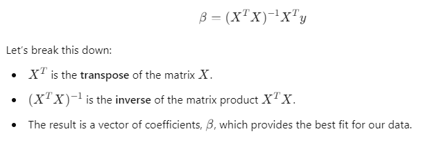
In this matrix equation, the key operations like transposition, matrix multiplication, and inversion all come from linear algebra for data science. These are essential tools in solving regression problems efficiently.
3. Step-by-Step Solution with Python and NumPy
Now let’s move to the Python implementation using NumPy. We’ll take a simple dataset and solve the linear regression problem step by step.
Example Data
We’ll use a small dataset of house sizes (in square feet) and their corresponding prices. Our goal is to predict the house price based on the size.
import numpy as np

# Size of the house (in square feet)
X = np.array([[1, 1500], [1, 2000], [1, 2500], [1, 3000], [1, 3500]])

# Price of the house (in dollars)
y = np.array([300000, 400000, 500000, 600000, 700000])
Here:
- X is our input matrix (we add a column of 1s to account for the intercept term).
- y is our target vector, the actual house prices.
Step 1: Transpose the Input Matrix
The first step is to compute the transpose of X. This operation flips the matrix over its diagonal, which will help us in the next step.
X_T = X.T
print(X_T)
Step 2: Matrix Multiplication
Next, we perform the matrix multiplication of X^T and X. This operation is at the heart of linear algebra for data science because it’s used in many machine learning algorithms to compute important values like covariance matrices.
X_T_X = np.dot(X_T, X)
print(X_T_X)
Step 3: Invert the Matrix
Now we need to compute the inverse of the matrix product X^T X. Matrix inversion is a critical operation in linear regression, and it’s where things get computationally heavy for larger datasets.
X_T_X_inv = np.linalg.inv(X_T_X)
print(X_T_X_inv)
Step 4: Calculate β (Coefficients)
Finally, we can calculate the coefficients β\betaβ by multiplying X_T_X^{-1}, X_T, and y together.
beta = np.dot(np.dot(X_T_X_inv, X_T), y)
print(beta)
The output will give us the values of the intercept and the slope. These are the parameters of the linear regression model.
4. Interpreting the Results
Once we’ve calculated the coefficients β, we can use them to make predictions for house prices based on their sizes. For example, to predict the price of a 2,750 square foot house:
house_size = 2750
predicted_price = beta[0] + beta[1] * house_size
print(predicted_price)
With the coefficients β\betaβ, you’ll see how simple it is to make predictions on new data points. This is a typical application of linear algebra for data science: solving real-world problems with mathematical tools.
5. Why This Matters
From personal experience, this process—though simple for small datasets—becomes more challenging as your data grows. When dealing with big data or high-dimensional datasets, matrix operations like inversion can become slow. That’s why understanding the underlying math and how libraries like NumPy handle these calculations is crucial. Linear algebra is not just an abstract concept but a powerful tool that can make or break your machine learning models.
Whether you’re working on small-scale problems or tackling large datasets, linear algebra for data science will always be at the core of your solutions. Knowing how to use these tools effectively will help you handle more complex problems down the road.
Practical Example: Implementing PCA with Scikit-Learn
Principal Component Analysis (PCA) is a powerful technique used in machine learning for dimensionality reduction. When you have a large dataset with many features, it can sometimes be difficult to visualize, analyze, or model. PCA helps by reducing the number of dimensions while preserving as much information as possible. In this guide, we will break down how to use Scikit-Learn to perform PCA and explain the math behind it in simple terms.
We’ll walk through a practical step-by-step guide that includes code snippets, mathematical concepts, and personal insights to make this topic more relatable. Along the way, I’ll highlight how PCA ties into linear algebra for data science, as it’s an important technique you’ll come across often.
1. What is PCA?
PCA is a method that transforms the data from its original high-dimensional space into a lower-dimensional space. The goal is to identify the principal components—new variables that capture the maximum variance in the data.
Here’s a simplified version of the mathematical process:
- Covariance matrix: PCA starts by calculating the covariance matrix of your data, which shows how much each variable varies with others.
- Eigenvectors and eigenvalues: It then computes the eigenvectors (directions of maximum variance) and eigenvalues (magnitudes of variance in those directions) from the covariance matrix.
- Projection: The data is projected onto the new principal components to create a lower-dimensional representation.
2. Why Use PCA for Dimensionality Reduction?
When working with large datasets, especially in data science applications, you may face the problem of having too many features or variables. This can lead to overfitting or slow down the training of your machine learning model. Dimensionality reduction techniques like PCA help:
- Simplify models without losing much information.
- Speed up training time.
- Reduce multicollinearity among features.
3. Step-by-Step Guide to Implementing PCA with Scikit-Learn
Let’s now go through the steps of implementing PCA using Scikit-Learn in Python. We’ll use the famous Iris dataset for this example, which contains data on different flower species and their features like sepal length, petal width, etc.
Step 1: Importing Required Libraries
First, you need to import the necessary libraries, including Scikit-Learn and NumPy.
import numpy as np
import matplotlib.pyplot as plt
from sklearn.decomposition import PCA
from sklearn.datasets import load_iris
from sklearn.preprocessing import StandardScaler
Step 2: Load the Data and Preprocess
PCA requires that the data be centered and scaled, meaning that each feature has a mean of 0 and unit variance. We’ll use StandardScaler to scale the features in the Iris dataset.
# Load the Iris dataset
data = load_iris()
X = data.data
y = data.target

# Standardize the data
scaler = StandardScaler()
X_scaled = scaler.fit_transform(X)
Step 3: Applying PCA
Now, we can apply PCA to reduce the number of dimensions. Let’s reduce it from 4 to 2, which allows us to visualize the data in two dimensions.
# Apply PCA
pca = PCA(n_components=2)
X_pca = pca.fit_transform(X_scaled)

# Output the explained variance
print(f"Explained variance ratio: {pca.explained_variance_ratio_}")
The explained variance ratio tells us how much of the total variance is captured by each principal component. It’s a good way to check how much information we are retaining after dimensionality reduction.
Step 4: Visualizing the Result
One of the best parts of PCA is that it allows us to visualize high-dimensional data in a lower-dimensional space. Below is a plot that shows the Iris data projected onto the first two principal components.
# Plot the PCA results
plt.figure(figsize=(8,6))
plt.scatter(X_pca[:, 0], X_pca[:, 1], c=y, cmap='viridis', edgecolor='k')
plt.xlabel('First Principal Component')
plt.ylabel('Second Principal Component')
plt.title('PCA on Iris Dataset')
plt.show()
You should see that the different species of flowers are grouped together, meaning that PCA has captured important patterns in the data even after reducing the dimensionality.
4. The Math Behind PCA: A Simplified Breakdown
The math behind PCA involves key concepts from linear algebra:
- Covariance Matrix: This is a square matrix that captures how each feature in the dataset correlates with the others. It’s calculated as:

- Eigenvectors and Eigenvalues: These are extracted from the covariance matrix. The eigenvectors represent the directions of maximum variance, and the eigenvalues represent the amount of variance along those directions.
PCA effectively rotates the data such that the most variance is captured in the first principal component, the second most variance in the second component, and so on.
This transformation is done using matrix multiplication, where the original data is projected onto the eigenvectors.
6. Summary of Key Points
- Principal Component Analysis (PCA) is a dimensionality reduction technique that transforms data into a lower-dimensional space by identifying the directions of maximum variance.
- PCA involves key linear algebra concepts such as covariance matrices, eigenvectors, and eigenvalues.
- The process can be implemented easily with Scikit-Learn in Python, making it accessible for data science tasks.
- PCA is especially useful in reducing the complexity of large datasets while retaining most of the important information.
- A key application of PCA is in visualizing high-dimensional data in a lower-dimensional space.
7. Code Snippet for Quick Reference
To summarize, here’s the full code for applying PCA to the Iris dataset:
import numpy as np
import matplotlib.pyplot as plt
from sklearn.decomposition import PCA
from sklearn.datasets import load_iris
from sklearn.preprocessing import StandardScaler

# Load and standardize the dataset
data = load_iris()
X = data.data
y = data.target
scaler = StandardScaler()
X_scaled = scaler.fit_transform(X)

# Apply PCA
pca = PCA(n_components=2)
X_pca = pca.fit_transform(X_scaled)

# Visualize the PCA result
plt.figure(figsize=(8,6))
plt.scatter(X_pca[:, 0], X_pca[:, 1], c=y, cmap='viridis', edgecolor='k')
plt.xlabel('First Principal Component')
plt.ylabel('Second Principal Component')
plt.title('PCA on Iris Dataset')
plt.show()

# Explained variance
print(f"Explained variance ratio: {pca.explained_variance_ratio_}")
Why PCA is Essential in Data Science
PCA is a must-have tool in the data science toolbox, especially when dealing with high-dimensional data. It simplifies datasets while retaining the most crucial information, making it easier to build models and interpret results. Understanding how linear algebra underpins PCA will make you a more effective practitioner, especially when working with large datasets or complex features.
Whether you’re applying PCA for visualization, noise reduction, or to improve model efficiency, it is an indispensable technique for modern machine learning.
If you’re serious about mastering linear algebra for data science, implementing PCA is a great starting point.
Conclusion
As we’ve seen in this second part, advanced linear algebra concepts like Singular Value Decomposition (SVD), tensors, and matrix factorization play a vital role in cutting-edge machine learning techniques. These methods power everything from recommendation systems to deep learning frameworks like TensorFlow and PyTorch.
Furthermore, the exploration of non-negative matrix factorization (NMF), quantum linear algebra, and neural networks highlights how new research continues to push the boundaries of what we can achieve with matrix-based operations. Whether you’re working on linear regression, implementing PCA, or developing the next generation of recommender systems, linear algebra remains a key tool for optimizing your models and improving computational efficiency.
By applying these powerful mathematical techniques in real-world scenarios, data scientists and engineers can unlock new levels of performance and scalability. As technology evolves, linear algebra will continue to be a crucial pillar for advancements in machine learning, AI, and big data.
FAQs
1. What is Singular Value Decomposition (SVD) and why is it important in data science?
Singular Value Decomposition (SVD) is a matrix factorization technique used to break down a matrix into simpler components. It’s crucial in data science for applications like recommendation systems, image compression, and natural language processing.
2. How are tensors used in machine learning?
Tensors are multi-dimensional arrays that extend the concept of matrices. They are essential in deep learning frameworks like TensorFlow and PyTorch for training neural networks by efficiently representing large datasets.
3. What is Non-Negative Matrix Factorization (NMF) and how is it applied in recommendation systems?
NMF is a matrix factorization method where the matrix elements are non-negative. It’s commonly used in recommendation systems to predict user preferences by decomposing the user-item interaction matrix.
4. How do linear regression models utilize matrices?
Linear regression models use matrices to represent datasets and perform calculations. Matrix multiplication is key in determining model parameters and making predictions efficiently.
External Resources
Applications of Linear Algebra Applied to Big Data Analytics
Machine Learning, Statistics, and Data Science” by David Barber
- This research paper discusses the interplay between linear algebra, statistics, and machine learning.
- Access the paper







Leave a Reply