Autoregressive Models for Time Series Predictions: A Comprehensive Guide
Introduction – Time Series Prediction using Autoregressive Models
Have you ever wondered how we can predict future events based on past data? Whether it’s forecasting the weather, stock prices, or even your favorite sports team’s performance, there’s a powerful approach called autoregressive models that can help. In this comprehensive guide, we’re going to explore how these models work and how you can use them for time series predictions.
Autoregressive models are like having a crystal ball that looks at the past to predict the future. They analyze patterns in data over time and use that information to forecast what’s coming next. The best part? You don’t need to be a data expert to understand them. We’ll explain it in a clear and simple way, with relatable examples to keep it engaging and fun.
So, if you’re curious about how to make more accurate predictions and want to learn a powerful tool that can help you do just that, stick around! By the end of this guide, you’ll have a solid grasp of autoregressive models and be ready to apply them to your own projects. Let’s get started!
Understanding Autoregressive Models
What are Autoregressive Models?
Autoregressive (AR) models are a type of statistical model that predicts future values in a time series data based on past values. In other words, they use the history of the data to forecast future outcomes.
Here’s a simple explanation:
- Time series data: A sequence of data points measured at regular time intervals (e.g., daily temperatures, stock prices, etc.).
- Autoregression: The model uses past values in the time series to predict future values.
- Regression: The model finds the best-fitting line (or curve) that describes the relationship between past and future values.
The AR model assumes that the current value of the time series is a function of previous values, and uses this relationship to make predictions. The model can be represented by the equation:
Where:
- Y(t) is the current value
- Y(t-1), Y(t-2), …, Y(t-p) are past values
- φ1, φ2, …, φp are model parameters
- ε(t) is the error term
AR models are widely used in finance, economics, weather forecasting, and other fields where time series data is common. They’re particularly useful for predicting continuous outcomes, like stock prices or temperatures, and can be extended to more complex models, like ARMA and ARIMA, to handle non-stationarity and seasonality.
How Autoregressive Models Generate Data
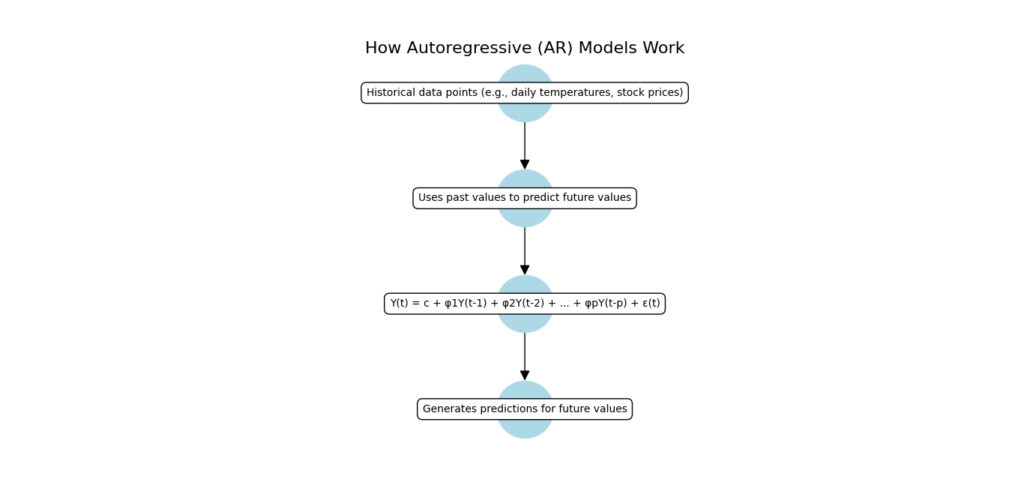
An Autoregressive (AR) model is a way to predict future values based on past values of a time series. It works using a specific equation that combines past data with some random noise. Here’s a step-by-step breakdown of how it functions:
1. The AR Model Equation
The equation for an AR model looks like this:
Let’s break down each part of this equation:
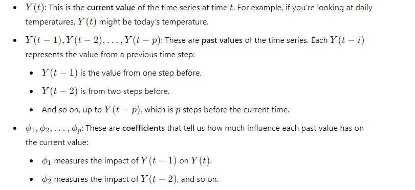
- These coefficients are determined during the model fitting process and show how strongly each past value affects the prediction.
- c: This is a constant value. It adjusts the overall level of the model to better fit the data. Think of it as a baseline value that helps the model align with the general trend of the data.
- ϵ(t): This is the error term or noise. It accounts for random variations that the model can’t predict. For instance, even if the model is very good at predicting, there will always be some unexpected fluctuations in real data, which are captured by this term.
2. How the AR Model Generates Predictions
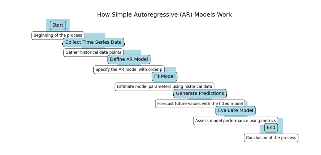
Here’s a step-by-step explanation of how an Autoregressive (AR) Model predicts future values based on past data:
1. Start with Historical Data
First, you need to gather the historical data for your time series. For example, if you’re trying to predict future temperatures, start by using the temperatures from previous days. This is your starting point for making predictions.
2. Apply the Model Equation
Next, you use the AR model equation to calculate the next value you want to predict. Here’s how you do it:
- Plug in the Past Values: Take the values from previous time steps (e.g., temperatures from the last few days).
- Use the Model Equation: For example, if you want to find the temperature for the next day, you use the equation:
- Y(t) is the most recent temperature.
- Y(t−1) is the temperature from the day before.
- And so on for as many past values as your model uses.
3. Add Random Noise
After calculating the predicted value, you need to add some random noise. This noise is represented by ϵ(t+1), and it accounts for:
- Unpredictable Variations: Real-world data often has random fluctuations that the model can’t always predict.
- Making Predictions Realistic: By adding this noise, your prediction becomes more realistic and reflects the fact that not all changes can be predicted from past data alone.
4. Repeat for Future Values
Once you have your predicted value:
- Update the Data: Use the newly predicted value as part of the data for making the next prediction. For example, if you predicted the temperature for tomorrow, use this prediction to help forecast the day after tomorrow.
- Continue the Process: Keep repeating this process to forecast further into the future. Each new prediction builds on the previous one, using the updated values from your model.
3. Why Randomness is Important
The error term ϵ(t) introduces a degree of randomness into the model. Without this, the data would follow a very smooth path, which is unrealistic for many real-world scenarios. By including this randomness, the model generates more realistic data that reflects the inherent variability in actual time series data.
4. Visualizing the Process
When you visualize the data generated by an AR model, you’ll see that it follows the general trend of the historical data but includes some random fluctuations. This helps in understanding how well the model replicates real-world data and makes future predictions.
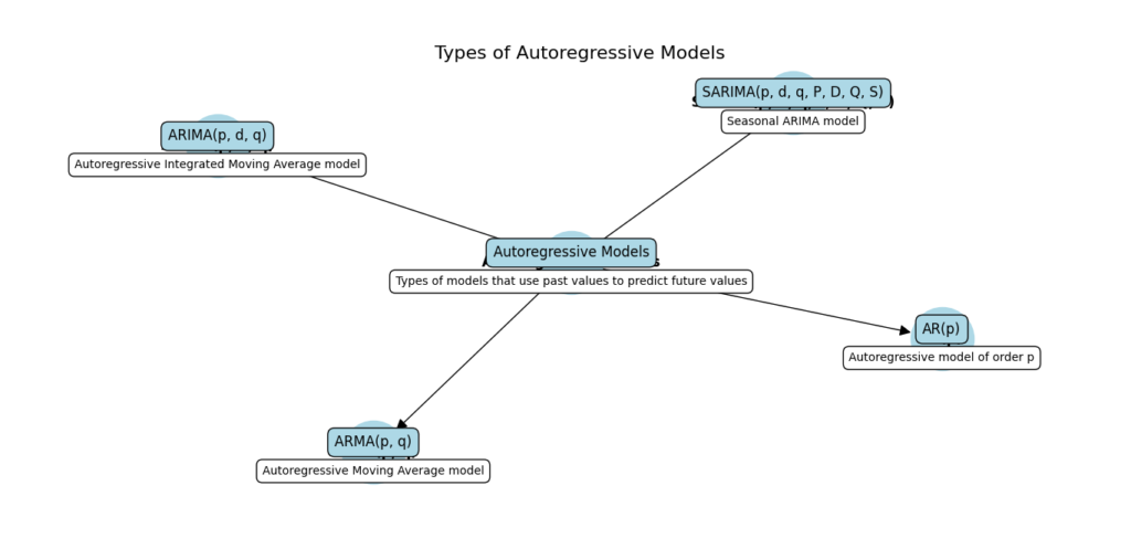
Types of Autoregressive Models
Simple Autoregressive (AR) Models
Simple Autoregressive (AR) models are a handy tool for predicting future values based on past data. Imagine you want to guess next month’s sales based on the sales from previous months. That’s exactly what AR models do! Let’s Explore how these models work and their key aspects.
Key Components
Lagged Values:
AR models look at past values, called lagged values, to make predictions. Think of it like looking at past trends to guess what might happen next. For instance, if you’re predicting sales for June, you might look at sales from May, April, and March.
Model Parameters (φ):
The model has parameters, often denoted as φ (phi), that define the relationship between past and future values. These parameters tell the model how much weight to give to each past value when making a prediction. For example, if φ1 is 0.5 and φ2 is 0.3, the model uses these weights to combine past values.
Order (p):
The order of an AR model, denoted as p, is the number of past values (lags) it uses. For example, an AR(1) model uses just the last value, while an AR(3) model uses the last three values. The choice of p depends on how far back you want to look when making predictions.
AR Model Equation
Here’s the basic equation for an AR model:
Where:
- Y(t) is the current value.
- Y(t-1), Y(t-2), …, Y(t-p) are the lagged values.
- φ1, φ2, …, φp are the model parameters.
- ε(t) is the error term (the part the model can’t predict).
- c is a constant term.
In simpler terms, to predict the current value Y(t), the model looks at past values Y(t-1), Y(t-2), …, Y(t-p), multiplies them by the parameters φ1, φ2, …, φp, adds them up along with a constant term c, and adds an error term ε(t).
Assumptions
Stationarity:
The time series should be stationary, meaning its statistical properties like mean and variance don’t change over time. This makes it easier to model and predict. If the data isn’t stationary, it can often be made so by differencing (subtracting the previous value from the current value).
Linearity:
The relationship between past and future values should be linear. This means if you plot the values, you should be able to draw a straight line through them (more or less). Non-linear relationships might require more advanced models.
Advantages
Simple to Implement:
AR models are easy to understand and set up. You don’t need advanced math skills to use them. Basic statistical knowledge is usually enough to get started.
Fast Computation:
These models run quickly on computers, even with large datasets. This efficiency makes them suitable for real-time applications where quick predictions are necessary.
Limitations
Assumptions:
AR models assume stationarity and linearity, which may not always be true. If your data has trends (like increasing sales over time) or seasonal patterns (like higher sales every December), you might need a more complex model, such as ARIMA or SARIMA.
Limited Flexibility:
AR models can only capture linear relationships. If your data has more complex patterns, AR models might not give the best predictions. In such cases, non-linear models or machine learning techniques might be more appropriate.
Autoregressive Moving Average (ARMA) Models
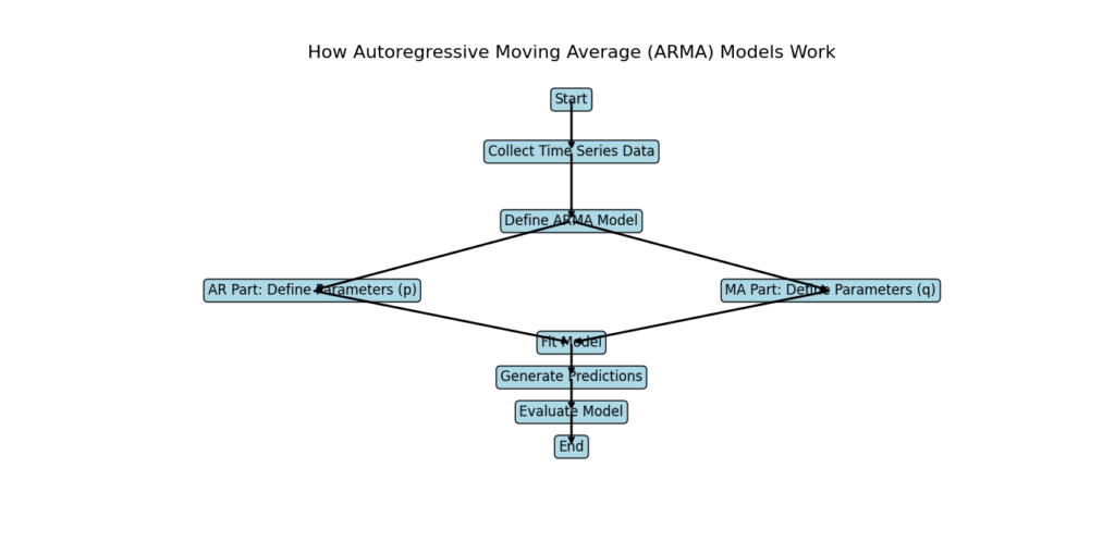
Autoregressive Moving Average (ARMA) models are powerful tools for predicting future values in a time series by combining two approaches: autoregressive (AR) and moving average (MA). Let’s Explore what ARMA models are and how they work.
Key Components
Autoregressive (AR) Component:
The AR part of the model uses past values to predict future values. It looks at how previous data points can influence what happens next. For example, if you’re predicting next month’s sales, you might look at the sales from the last few months.
Moving Average (MA) Component:
The MA part uses errors (also known as residuals) from past predictions to improve future predictions. If there was a big error in predicting last month’s sales, the model takes that into account to adjust its future predictions.
Model Parameters (φ and θ):
The model has parameters, denoted as φ (phi) for the AR part and θ (theta) for the MA part. These parameters define the relationship between past values, past errors, and future values. They basically tell the model how much weight to give to each past value and error.
Order (p, q):
The order of the ARMA model is denoted as (p, q). The p is the number of past values (lags) used in the AR part, and q is the number of past errors used in the MA part. For example, an ARMA(2, 1) model uses the last two values and the last error.
ARMA Model Equation
Here’s the basic equation for an ARMA model:
Where:
- Y(t) is the current value.
- Y(t-1), Y(t-2), …, Y(t-p) are the lagged values.
- ε(t-1), ε(t-2), …, ε(t-q) are the errors from past predictions.
- φ1, φ2, …, φp are the AR parameters.
- θ1, θ2, …, θq are the MA parameters.
- ε(t) is the error term (the part the model can’t predict).
- c is a constant term.
In simple terms, to predict the current value Y(t), the model looks at past values Y(t-1), Y(t-2), …, Y(t-p) and past errors ε(t-1), ε(t-2), …, ε(t-q), multiplies them by the parameters φ1, φ2, …, φp and θ1, θ2, …, θq, adds them up along with a constant term c, and adds an error term ε(t).
Assumptions
Stationarity:
The time series should be stationary, meaning its statistical properties like mean and variance don’t change over time. This makes it easier to model and predict. If the data isn’t stationary, it can often be made so by differencing (subtracting the previous value from the current value).
Linearity:
The relationship between past values, past errors, and future values should be linear. This means if you plot the values and errors, you should be able to draw a straight line through them (more or less).
Advantages
Flexibility:
ARMA models can handle both autoregressive and moving average effects, making them more flexible. They can capture patterns that pure AR or pure MA models might miss.
Improved Accuracy:
By combining AR and MA components, ARMA models can often provide more accurate forecasts than using AR or MA models alone. They take into account more information from the past data.
Limitations
Complexity:
ARMA models can be more difficult to implement and interpret than AR or MA models. Setting the right order (p, q) and estimating the parameters can be challenging.
Overfitting:
ARMA models can suffer from overfitting if the order (p, q) is too high. This means the model fits the past data too closely and may not perform well on new data.
Autoregressive Integrated Moving Average (ARIMA) Models
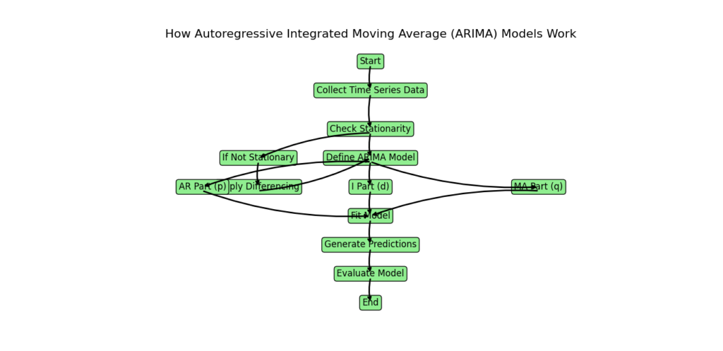
Autoregressive Integrated Moving Average (ARIMA) models are a popular tool for forecasting time series data. They are particularly useful when your data shows patterns over time that aren’t consistent or when the data changes in a way that makes it hard to predict future values.
Here’s a simple Explanation of ARIMA models:
Must Read
- PyTorch Debugging Checklist: A Systematic Framework to Fix Models That Won’t Learn
- Why sorted() Is Safer Than list.sort() in Production Python Systems
- Monotonic Sequence in Python: 7 Practical Methods With Edge Cases, Interview Tips, and Performance Analysis
- How to Check if Dictionary Values Are Sorted in Python
- Check If a Tuple Is Sorted in Python — 5 Methods Explained
Key Components
- Autoregressive (AR) Component: This part looks at past values of the series to predict future values. For example, if you’re predicting next month’s sales, you might use the sales figures from the past few months.
- Integrated (I) Component: This part involves differencing, which means subtracting previous values from the current value to make the data more stable (stationary). Stationary data means the properties like mean and variance don’t change over time, which makes it easier to model.
- Moving Average (MA) Component: This part uses past errors (the difference between predicted and actual values) to correct future predictions. It helps to smooth out the prediction errors.
Model Parameters
The ARIMA model has three key parameters:
- φ (phi): These are parameters for the autoregressive part. They determine how much past values affect future values.
- d: This is the number of differencing steps needed to make the series stationary.
- θ (theta): These are parameters for the moving average part. They control how past errors are used in the prediction.
Order of the Model
The order of an ARIMA model is written as (p, d, q):
- p: The number of past values used (autoregressive part).
- d: The number of differencing steps.
- q: The number of past errors used (moving average part).
ARIMA Model Equation
The basic form of the ARIMA model can be written as:
Where:
- Δ^dY(t): The differenced time series data.
- Y(t-1), …, Y(t-p): Past values of the series.
- ε(t-1), …, ε(t-q): Past errors.
- φ1, …, φp: Parameters for the autoregressive part.
- θ1, …, θq: Parameters for the moving average part.
- ε(t): The current error term.
Assumptions
For the ARIMA model to work well:
- Stationarity: The data should be stationary after differencing.
- Linearity: The relationships in the data should be linear.
Advantages
- Handles Non-Stationarity: ARIMA models can manage data that changes over time.
- Flexibility: They can deal with both past values and past errors to improve predictions.
Limitations
- Complexity: Setting up and understanding ARIMA models can be tricky compared to simpler models.
- Overfitting: If the model parameters (p, d, q) are set too high, the model might fit the training data too closely, which can hurt its performance on new data.
ARIMA models are powerful tools for time series forecasting, but they need careful tuning and understanding to use effectively.
Seasonal Autoregressive Integrated Moving-Average (SARIMA) Models
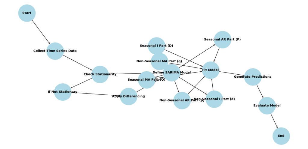
Seasonal Autoregressive Integrated Moving-Average (SARIMA) models are an advanced version of ARIMA models designed to handle seasonality in time series data. Seasonality refers to patterns that repeat at regular intervals, like monthly sales spikes during the holiday season.
Here’s a Explanation of SARIMA models:
Key Components
- Autoregressive (AR) Component: This part uses past values of the series to forecast future values. For example, if you’re predicting next quarter’s sales, you use sales data from previous quarters.
- Integrated (I) Component: This involves differencing the data to make it stationary. Stationary data means the statistical properties like mean and variance are constant over time, which helps in modeling.
- Moving Average (MA) Component: This part accounts for past errors (the differences between actual and predicted values) to improve future forecasts. It helps to adjust predictions based on previous mistakes.
- Seasonal (S) Component: This component is specifically for handling seasonality. It uses seasonal differencing to adjust for repeating patterns at specific intervals, like yearly or monthly.
Model Parameters
The SARIMA model has six key parameters:
- φ (phi): These are parameters for the autoregressive part.
- d: The number of differencing steps needed to make the data stationary.
- θ (theta): Parameters for the moving average part.
- Φ (Phi): Parameters for the seasonal autoregressive part.
- D: The number of seasonal differencing steps.
- Q: Parameters for the seasonal moving average part.
Order of the Model
The SARIMA model is denoted as (p, d, q, P, D, Q):
- p: Number of past values used (autoregressive part).
- d: Number of differencing steps.
- q: Number of past errors used (moving average part).
- P: Number of seasonal past values used.
- D: Number of seasonal differencing steps.
- Q: Number of seasonal past errors used.
SARIMA Model Equation
The equation for SARIMA can be expressed as:
Where:
- Δ^dΔ_s^DY(t): The seasonally differenced time series.
- Y(t-1), …, Y(t-p): Past values of the series.
- ε(t-1), …, ε(t-q): Past errors.
- Φ1, …, ΦP: Parameters for the seasonal autoregressive part.
- D: Number of seasonal differencing steps.
- Q: Parameters for the seasonal moving average part.
- ε(t): The current error term.
Assumptions
For SARIMA models to work well:
- Stationarity: The data should be stationary after seasonal differencing.
- Linearity: The relationships in the data should be linear.
Advantages
- Handles Seasonality: SARIMA models are great for dealing with repeating patterns or seasonal changes in time series data.
- Flexibility: They can handle both regular and seasonal patterns, as well as errors in predictions.
Limitations
- Complexity: SARIMA models can be more complex to set up and interpret compared to simpler models like ARIMA.
- Overfitting: If the model parameters (p, d, q, P, D, Q) are set too high, the model might fit the training data too closely, which can make it less accurate for new data.
Practical Applications of Autoregressive (AR) Models
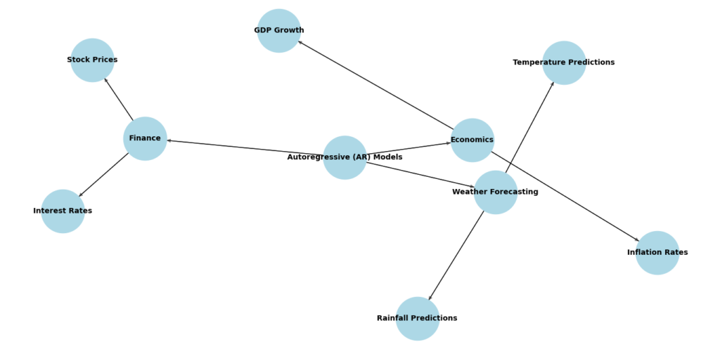
Autoregressive (AR) models are powerful tools that find applications in many areas. Here’s a detailed look at how they are used in various fields:
1. Financial Forecasting with Autoregressive Models
In the finance sector, AR models are used for:
- Stock Prices: Predicting future stock prices based on past performance.
- Portfolio Optimization: Helping investors build a balanced portfolio by analyzing past returns.
- Risk Management: Assessing the risk of financial assets by looking at historical data.
- Algorithmic Trading: Designing trading strategies that use past market data to make trading decisions.
2. Economics
AR models play a crucial role in economics by:
- GDP Forecasting: Predicting future Gross Domestic Product (GDP) based on past economic data.
- Inflation Prediction: Estimating future inflation rates using historical inflation data.
- Econometric Modeling: Building models that explain economic relationships and predict future trends.
3. Weather Prediction Using Autoregressive Models
Weather forecasting benefits from AR models in:
- Temperature Prediction: Forecasting future temperatures based on past weather data.
- Precipitation Prediction: Estimating future rainfall amounts.
- Wind Speed Prediction: Predicting future wind speeds using historical data.
4. Autoregressive Models in Sales and Demand Forecasting
In sales, AR models are used for:
- Demand Planning: Predicting future product demand to ensure adequate supply.
- Inventory Management: Managing inventory levels based on past sales data.
- Revenue Prediction: Estimating future revenue based on historical sales figures.
5. Traffic Prediction
Traffic management uses AR models for:
- Predicting traffic patterns and flow on roads.
- Congestion Analysis: Analyzing traffic congestion and suggesting improvements.
- Route Optimization: Finding the best routes to avoid traffic jams.
6. Energy Forecasting
Energy companies use AR models for:
- Electricity Demand: Forecasting future electricity usage to balance supply and demand.
- Energy Consumption: Predicting overall energy consumption.
- Renewable Energy Prediction: Estimating the output from renewable sources like wind and solar.
7. Agriculture
In agriculture, AR models help with:
- Crop Yield Prediction: Estimating future crop yields based on past data.
- Weather-Based Farming: Using weather forecasts to plan farming activities.
- Agricultural Economics: Analyzing economic trends in agriculture.
8. Healthcare
Healthcare applications of AR models include:
- Disease Forecasting: Predicting future disease outbreaks based on past trends.
- Patient Outcomes Prediction: Estimating future patient health outcomes.
- Resource Allocation: Planning and managing healthcare resources effectively.
9. Marketing
In marketing, AR models assist with:
- Customer Behavior Analysis: Understanding past customer behavior to predict future actions.
- Market Trend Prediction: Forecasting future market trends.
- Campaign Optimization: Improving marketing campaigns by analyzing past performance.
10. Supply Chain Management
AR models are valuable in supply chain management for:
- Demand Forecasting: Predicting future demand for products.
- Inventory Optimization: Managing inventory levels to avoid shortages or overstocking.
- Logistics Planning: Planning transportation and logistics based on past data.
When AR Models Are Useful
AR models are particularly effective when:
- Strong Temporal Dependence: The data shows a clear relationship over time.
- Past Predicts Future: Historical data can reliably forecast future values.
- Patterns, Trends, or Seasonality: The data exhibits regular patterns or trends.
By using AR models, organizations can make better decisions, optimize resources, and improve the accuracy of their forecasts. These models help in understanding past data trends and making informed predictions about the future.
Getting Started with Python for Time Series Analysis
Building a Simple Weather Forecast using Seasonal Autoregressive Integrated Moving-Average (SARIMA) Model
Weather forecasting is a crucial aspect of many industries, from agriculture to event planning. One effective approach to forecasting time-series data like temperature is the Seasonal Autoregressive Integrated Moving-Average (SARIMA) model. SARIMA extends the ARIMA model by incorporating seasonal effects, making it well-suited for data with periodic patterns.
Here Let’s explore how to build a simple weather forecasting model using SARIMA.
1. Importing Libraries
import pandas as pd
import numpy as np
import matplotlib.pyplot as plt
from statsmodels.tsa.statespace.sarimax import SARIMAX
from datetime import datetime
- pandas: For handling data structures and time series data.
- numpy: For numerical operations and generating sample data.
- matplotlib.pyplot: For plotting graphs.
- statsmodels.tsa.statespace.sarimax: For fitting the SARIMA model.
- datetime: For handling date and time information.
2. Generating Sample Data
dates = pd.date_range(start='2000-01-01', periods=288, freq='ME')  # Monthly End frequency
temperature_data = np.sin(np.linspace(0, 3.14 * 6, 288)) + np.random.normal(scale=0.5, size=288)
df_temperature = pd.DataFrame({'Temperature': temperature_data}, index=dates)
pd.date_range: Creates a range of dates starting from January 2000, with 288 periods (months), ending at December 2023.np.sin: Generates sinusoidal data to simulate seasonal variations in temperature.np.random.normal: Adds random noise to the data.pd.DataFrame: Creates a DataFrame with the generated temperature data and dates as the index.
3. Resampling and Interpolating Data
df_resampled = df_temperature.resample('ME').interpolate(method='cubic')
resample('ME'): Resamples the data to monthly frequency using the end of the month (‘ME’).interpolate(method='cubic'): Interpolates missing values using cubic interpolation.
4. Defining the SARIMA Model
exog_data = pd.DataFrame({'Weather_Pattern': np.random.normal(scale=0.1, size=len(df_resampled))}, index=df_resampled.index)
model = SARIMAX(df_resampled['Temperature'],
                 exog=exog_data,
                 order=(2, 1, 2),          # ARIMA order
                 seasonal_order=(1, 1, 1, 12),  # SARIMA seasonal order
                 enforce_stationarity=False,
                 enforce_invertibility=False)
Explanation:
Creating Exogenous Variables
exog_data = pd.DataFrame({'Weather_Pattern': np.random.normal(scale=0.1, size=len(df_resampled))}, index=df_resampled.index)
pd.DataFrame: This function creates a DataFrame, which is a table of data.
'Weather_Pattern': This is the name of the new column we’re adding. It represents an external factor that might affect the temperature, like a weather pattern.
np.random.normal(scale=0.1, size=len(df_resampled)): Generates random numbers with a normal (bell curve) distribution. These numbers simulate the effect of the weather pattern.
scale=0.1: Determines how spread out the numbers are. Smaller values mean the numbers are closer to the mean.size=len(df_resampled): The number of random numbers generated is the same as the number of data points in your temperature series.
index=df_resampled.index: Sets the same date index for this new DataFrame as the temperature data, so it aligns correctly.
Defining the SARIMA Model
model = SARIMAX(df_resampled['Temperature'],
                 exog=exog_data,
                 order=(2, 1, 2),          # ARIMA order
                 seasonal_order=(1, 1, 1, 12),  # SARIMA seasonal order
                 enforce_stationarity=False,
                 enforce_invertibility=False)
SARIMAX: This function from the statsmodels library defines a SARIMA model. It helps us forecast future values based on historical data.
df_resampled['Temperature']: This is the main data you’re using for the model, which is the temperature data.
exog=exog_data: This adds the external factor (weather pattern) to the model. It helps the model take into account external influences.
order=(2, 1, 2):
2(AR order): The number of past values the model will use to predict future values.1(I order): The number of times the data will be differenced to make it stationary. This means adjusting the data to remove trends or seasonality.2(MA order): The number of past prediction errors used to improve future predictions.
seasonal_order=(1, 1, 1, 12):
1(Seasonal AR order): The number of past seasonal values used to predict future values.1(Seasonal I order): The number of times the data will be differenced seasonally to make it stationary.1(Seasonal MA order): The number of past seasonal errors used to improve predictions.12: The number of periods in a season. For monthly data with yearly seasonality, this is set to 12.
enforce_stationarity=False: Allows the model to use non-stationary data. Normally, you want data to be stationary (no trends) for better results, but this setting allows for some flexibility.
enforce_invertibility=False: Allows the model to use non-invertible data. This setting gives some leeway in handling data that doesn’t strictly meet the invertibility condition.
5. Fitting the Model
# Fit the model
results = model.fit()
Explanation:
- Fitting the Model
model.fit(): This command tells the SARIMA model to fit itself to the data we provided. It uses the historical temperature data and the external factor (weather pattern) to learn patterns and relationships.results: This variable will store the results of the fitting process, including model parameters and diagnostic information.
Output:
When you run the fitting process, you see output related to the optimization algorithm used to find the best model parameters. Here’s a simplified breakdown of what the output means:
RUNNING THE L-BFGS-B CODE

           * * *

Machine precision = 2.220D-16
 N =            8     M =           10

At X0         0 variables are exactly at the bounds

At iterate    0    f=  1.02232D+00    |proj g|=  8.02612D-01

...

Tit   = total number of iterations
Tnf   = total number of function evaluations
Tnint = total number of segments explored during Cauchy searches
Skip  = number of BFGS updates skipped
Nact  = number of active bounds at final generalized Cauchy point
Projg = norm of the final projected gradient
F     = final function value

           * * *

   N    Tit     Tnf  Tnint  Skip  Nact     Projg        F
    8     33     40      1     0     0   2.588D-05   7.922D-01
  F =  0.79216447337016527
Explanation
Machine Precision: Indicates the numerical precision used in calculations. It’s a measure of how accurately the model’s calculations are performed.
N = 8: Number of model parameters being estimated.
M = 10: Number of variables involved in the optimization process.
At X0: This refers to the initial state of the optimization process where no parameters have yet been adjusted.
At iterate 0: Shows the progress of the optimization at the start (iteration 0).
- f= 1.02232: The initial value of the objective function (a measure of how well the model fits the data).
- |proj g|= 0.802612: The norm of the gradient (a measure of how much the function value is expected to change).
Tit = total number of iterations: The total number of times the optimization process has updated the model parameters.
Tnf = total number of function evaluations: The total number of times the objective function has been calculated during the optimization.
Tnint = total number of segments explored during Cauchy searches: The number of segments considered during a specific search method used in optimization.
Skip = number of BFGS updates skipped: Indicates how many updates were skipped in the optimization algorithm. BFGS is a method used for optimization.
Nact = number of active bounds at final generalized Cauchy point: The number of parameter bounds that were active at the end of the optimization.
Projg = norm of the final projected gradient: The final measure of the gradient’s norm, which should be close to zero for a good fit.
F = final function value: The final value of the objective function after fitting. This is a key measure of the model’s performance.
F = 0.79216447337016527: The final value of the objective function. A lower value generally indicates a better fit to the data.
6. Printing the Model Summary
print(results.summary())
results.summary(): Displays a summary of the fitted model, including coefficients, standard errors, and statistical tests.
Output: SARIMAX Results
After fitting the SARIMA model, you receive a summary of the results. Here’s a detailed breakdown of the key components of the output:
SARIMAX Results Summary
SARIMAX Results
============================================================================================
Dep. Variable:                          Temperature   No. Observations:                  288
Model:             SARIMAX(2, 1, 2)x(1, 1, [1], 12)   Log Likelihood                -228.143
Date:                              Mon, 29 Jul 2024   AIC                            472.287
Time:                                      10:58:02   BIC                            500.772
Sample:                                  01-31-2000   HQIC                           483.738
                                       - 12-31-2023
Covariance Type:                                opg
Dep. Variable: Temperature
- Temperature: The dependent variable modeled is temperature data.
No. Observations: 288
- 288: Number of monthly temperature data points used.
Model: SARIMAX(2, 1, 2)x(1, 1, [1], 12)
- SARIMAX(2, 1, 2): Non-seasonal ARIMA order (p=2, d=1, q=2).
- x(1, 1, [1], 12): Seasonal order (P=1, D=1, Q=1, S=12 for monthly seasonality).
Log Likelihood: -228.143
- -228.143: Log likelihood value, where higher (less negative) values indicate a better fit.
Date: Mon, 29 Jul 2024
- 29 Jul 2024: Date of model fitting.
Time: 10:58:02
- 10:58:02: Time of model fitting completion.
AIC: 472.287
- AIC (Akaike Information Criterion): Model quality measure, where lower values are better.
BIC: 500.772
- BIC (Bayesian Information Criterion): Similar to AIC, with a penalty for the number of parameters. Lower values are better.
Sample: 01-31-2000 – 12-31-2023
- 01-31-2000 – 12-31-2023: Data period used for modeling.
HQIC: 483.738
- HQIC (Hannan-Quinn Information Criterion): Another model quality measure, where lower values indicate a better fit.
Covariance Type: opg
- opg (Outer Product of Gradients): Method used to estimate the covariance matrix of parameter estimates.
Key Points:
- SARIMAX model includes non-seasonal and seasonal components for temperature data patterns.
- Information Criteria (AIC, BIC, HQIC) evaluate model performance and complexity, with lower values indicating better fits.
- Log Likelihood measures model fit quality, with higher values indicating a better fit.
6. Printing the Model Summary
print(results.summary())
results.summary(): Displays a summary of the fitted model, including coefficients, standard errors, and statistical tests.
Output
                     coef    std err          z      P>|z|      [0.025      0.975]
-----------------------------------------------------------------------------------
Weather_Pattern    -0.1583      0.294     -0.539      0.590      -0.734       0.417
ar.L1              -1.1377      0.076    -15.011      0.000      -1.286      -0.989
ar.L2              -0.2183      0.080     -2.736      0.006      -0.375      -0.062
ma.L1               0.3249   1827.065      0.000      1.000   -3580.656    3581.306
ma.L2              -0.6751   1233.429     -0.001      1.000   -2418.152    2416.802
ar.S.L12            0.0850      0.081      1.045      0.296      -0.074       0.244
ma.S.L12           -0.9036      0.072    -12.549      0.000      -1.045      -0.762
sigma2              0.3056    558.345      0.001      1.000   -1094.030    1094.641
===================================================================================
The table presents the results of the SARIMA model fit, showing the estimated coefficients and their statistical significance.
Sample Output Explanation:
coef: Coefficients for each parameter in the model.std err: Standard errors of the coefficients.zandP>|z|: Test statistics and p-values for the coefficients.sigma2: Variance of the residuals.AIC,BIC,HQIC: Information criteria used for model selection.
7. Generating Forecasts
forecast_period = 12 * 35  # Forecasting 35 years monthly
forecast_dates = pd.date_range(start=df_resampled.index[-1] + pd.DateOffset(months=1), periods=forecast_period, freq='ME')
forecast_exog = pd.DataFrame({'Weather_Pattern': np.random.normal(scale=0.1, size=forecast_period)}, index=forecast_dates)
forecast = results.get_forecast(steps=forecast_period, exog=forecast_exog)
forecast_df = forecast.conf_int()
forecast_period: Number of periods to forecast (35 years of monthly data).forecast_dates: Creates future dates for forecasting.forecast_exog: Generates future values for the exogenous variable.results.get_forecast(): Generates forecasted values.forecast.conf_int(): Gets the confidence intervals for the forecasts.
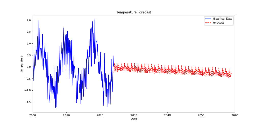
8. Adding Forecasted Values and Plotting
Let’s go through the steps involved in adding the forecasted values to our DataFrame and plotting the results.
Adding Forecasted Values
forecast_df['Forecast'] = forecast.predicted_mean
forecast_df.index = forecast_dates
- forecast_df[‘Forecast’] = forecast.predicted_mean: This line adds the forecasted temperature values to the
forecast_dfDataFrame. Thepredicted_meancontains the forecasted values generated by our SARIMA model. - forecast_df.index = forecast_dates: This sets the index of
forecast_dftoforecast_dates, which are the dates corresponding to our forecast period.
Plotting the Data
plt.figure(figsize=(12, 6))

# Plot historical data
plt.plot(df_resampled.index, df_resampled['Temperature'], label='Historical Data', color='blue')

# Plot forecasted data
plt.plot(forecast_df.index, forecast_df['Forecast'], label='Forecast', color='red', linestyle='--')

# Set plot title and labels
plt.title('Temperature Forecast')
plt.xlabel('Date')
plt.ylabel('Temperature')

# Show legend
plt.legend()

# Set x-axis limits for better visualization
plt.xlim(pd.Timestamp('2000-01-01'), pd.Timestamp('2060-01-01'))

# Show plot
plt.show()
Explanation
- plt.figure(figsize=(12, 6)): This initializes a new figure with a specified size of 12 inches by 6 inches. This helps in creating a plot that is large enough for clear visualization.
- plt.plot(df_resampled.index, df_resampled[‘Temperature’], …): This line plots the historical temperature data.
df_resampled.indexprovides the dates, anddf_resampled['Temperature']provides the corresponding temperature values. - label=’Historical Data’: This sets the label for the historical data, which will be used in the legend.
- color=’blue’: This sets the color of the historical data line to blue
- plt.plot(forecast_df.index, forecast_df[‘Forecast’], …): This line plots the forecasted temperature data.
forecast_df.indexprovides the forecast dates, andforecast_df['Forecast']provides the forecasted temperature values. - label=’Forecast’: This sets the label for the forecasted data, which will be used in the legend.
- color=’red’: This sets the color of the forecasted data line to red.
- linestyle=’–‘: This sets the line style to dashed, differentiating it from the solid historical data line.
- plt.title(‘Temperature Forecast’): This sets the title of the plot.
- plt.xlabel(‘Date’): This sets the label for the x-axis.
- plt.ylabel(‘Temperature’): This sets the label for the y-axis.
- plt.legend(): This displays the legend on the plot, helping to identify the historical and forecasted data lines.
- plt.xlim(pd.Timestamp(‘2000-01-01’), pd.Timestamp(‘2060-01-01’)): This sets the limits for the x-axis, ensuring that the plot shows data from January 1, 2000, to January 1, 2060.
- plt.show(): This renders the plot, making it visible
Output
Challenges and Limitations of Autoregressive Models
Common Pitfalls in Autoregressive Modeling
Every model has its challenges. Autoregressive models are no exception. Two of the most common issues are overfitting and underfitting. Overfitting happens when a model learns the details and noise in the training data too well. It performs great on the training data but poorly on new, unseen data. To avoid overfitting, you can:
- Simplify the model by reducing the number of parameters.
- Use cross-validation to ensure the model performs well on different subsets of the data.
- Regularize the model to penalize overly complex solutions.
Underfitting, on the other hand, occurs when a model is too simple to capture the underlying pattern in the data. It performs poorly on both training and test data. To prevent underfitting, you can:
- Add more relevant features to the model.
- Increase the complexity of the model by using a higher-order autoregressive model.
- Ensure the model is correctly specified and includes all important lagged variables.
Limitations of Autoregressive Models
Autoregressive models are powerful tools, but they aren’t always the best choice for every scenario. Here are some limitations to consider:
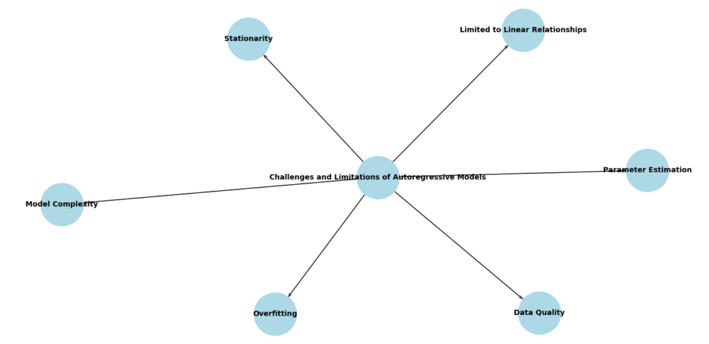
- Assumption of Stationarity: These models assume that the statistical properties of the series, like mean and variance, are constant over time. Many real-world time series, such as stock prices or weather data, are not stationary.
- Lag Selection: Choosing the appropriate number of lags is crucial. Too few lags can lead to underfitting, while too many can cause overfitting.
- Linear Relationships: Autoregressive models assume a linear relationship between the current value and its past values. This might not capture more complex, nonlinear patterns present in the data.
When facing these limitations, you might want to consider other models, such as:
- Moving Average (MA) Models: These models focus on the past errors rather than past values.
- ARIMA Models: Combining autoregressive and moving average models, ARIMA can handle non-stationary data by including differencing.
- SARIMA Models: Extending ARIMA by adding seasonal components to handle periodic patterns in the data.
Future Trends in Autoregressive Modeling
Emerging Techniques and Innovations
The world of autoregressive models is always evolving. Here are some of the latest innovations:
- Hybrid Models: These combine traditional statistical models with machine learning approaches, like deep learning, to capture complex patterns in the data.
- State Space Models: These models provide a flexible framework for time series analysis, accommodating a wide range of assumptions and data structures.
- Machine Learning Integration: Incorporating techniques like neural networks and ensemble learning can enhance the predictive power of autoregressive models.
Conclusion
In this guide, we’ve explored autoregressive models and their role in time series predictions. We started by understanding the basics of these models, including how they use past data to forecast future values. We then walked through practical examples and discussed how to set up these models for effective forecasting.
We covered the strengths of autoregressive models, such as their ability to handle historical data and make predictions based on patterns. We also addressed their limitations, including challenges like stationarity and lag selection.
Finally, we looked at some of the common pitfalls in using autoregressive models, such as overfitting and underfitting, and how to avoid them. We also discussed when it might be better to consider other modeling approaches or combine autoregressive models with newer techniques.
By understanding these concepts, you are now better equipped to use autoregressive models effectively in your own projects. Remember, no single model is perfect for every situation. The key is to choose the right approach based on your data and goals, and to keep exploring and learning as new methods and techniques emerge.
Apply what you’ve learned here, and you’ll be well on your way to making accurate and insightful time series predictions.
FAQs
What is an autoregressive model?
An autoregressive (AR) model is a type of statistical model used to predict future values based on past values in a time series. It uses the principle that past data points can help forecast future ones.
How does an autoregressive model work?
An autoregressive model works by regressing the current value of a time series on its previous values. For example, an AR(1) model predicts the next value based on just the most recent past value, while an AR(p) model uses the last p values.
What are the key parameters in an autoregressive model?
The key parameters in an autoregressive model include:
- Order (p): The number of previous time points used in the model.
- Coefficients: These are weights assigned to past values, determining their influence on the prediction.
What is the difference between AR and ARMA models?
An AR (Autoregressive) model uses only past values to make predictions, while an ARMA (Autoregressive Moving Average) model combines autoregressive terms with moving average terms, which include past forecast errors.
When should I use an autoregressive model?
Autoregressive models are best used when you have time series data that shows a clear pattern or trend over time. They are effective for short-term forecasting and can be used in various fields like finance, weather forecasting, and economics.
How can I improve my autoregressive model?
To improve your autoregressive model, you can:
- Analyze residuals: Check if the residuals (errors) are random and follow a normal distribution.
- Adjust the order: Test different values for the model’s order (p) to find the best fit.
- Consider other models: If an AR model isn’t giving good results, explore models like ARMA or ARIMA.
External Resources
- Autoregressive Models – StatsModels Documentation
- Offers comprehensive documentation and tutorials on autoregressive models using StatsModels in Python.
- Introduction to Time Series Analysis – University of Washington
- An educational resource with lectures and notes on time series analysis, including autoregressive models.
- Time Series Forecasting with ARIMA Models – R Documentation
- Official R documentation for ARIMA models, useful for understanding autoregressive approaches in forecasting.





Leave a Reply