

Best Python Libraries for Statistical Analysis: 6 Hidden Gems You Should Know
Introduction
Why Python is the Best Choice for Statistical Analysis
Python is one of the best tools for statistical analysis. Because it’s easy to use and has powerful libraries. Most data scientists work with NumPy, pandas, and SciPy, but there are many hidden Python libraries for statistical analysis.
If you need to do hypothesis testing, Bayesian analysis, time series analysis, or survival analysis, you don’t have to write complex code from scratch. There are special Python libraries that can help with statistical modeling and data cleaning, making your work faster.
In this post, we’ll look at six lesser-known Python libraries that can save you time and make statistical analysis simpler. Whether you’re working with Bayesian statistics, time series forecasting, or survival analysis, these libraries will help you get better results with less effort.
Let’s check out the best Python libraries for statistical analysis that you might not have heard of—but should definitely use!
The 6 Best Python Libraries for Statistical Analysis

Pingouin – Hypothesis Testing Made Simple
Statistical analysis is a big part of working with data, and one of the most common tasks is hypothesis testing—checking whether patterns in data are real or just random chance. Most people use SciPy for this, but there’s a hidden Python library that makes things much easier: Pingouin.
With Pingouin, you can perform complex statistical tests quickly and accurately, without writing long formulas or handling messy calculations yourself. It’s one of the best Python libraries for statistical analysis, especially if you need to run:
- Hypothesis testing (checking if differences between groups are real)
- Bayesian analysis (estimating probabilities instead of simple yes/no answers)
- Time series analysis (analyzing data that changes over time)
- Survival analysis (predicting when events, like failure or death, will happen)
- Data cleaning (handling missing values and errors)
Let’s break down hypothesis testing and see how Pingouin makes it easier with real examples.
What is Hypothesis Testing?
Whenever we analyze data, we usually have a question in mind:
- Does a new drug improve patient health?
- Are students who study longer getting better test scores?
- Is one marketing campaign performing better than another?
To answer these questions, we use hypothesis testing. This is a way to compare two ideas:
- Null Hypothesis (H₀): No real difference or effect exists.
- Alternative Hypothesis (H₁): There is a real difference or effect.
We calculate a p-value to see which hypothesis is more likely:
✔ If p < 0.05, we reject H₀ (meaning the difference is probably real).
✔ If p ≥ 0.05, we fail to reject H₀ (meaning the difference might be due to random chance).
Manually calculating p-values and running statistical tests can be difficult. This is where Pingouin helps!
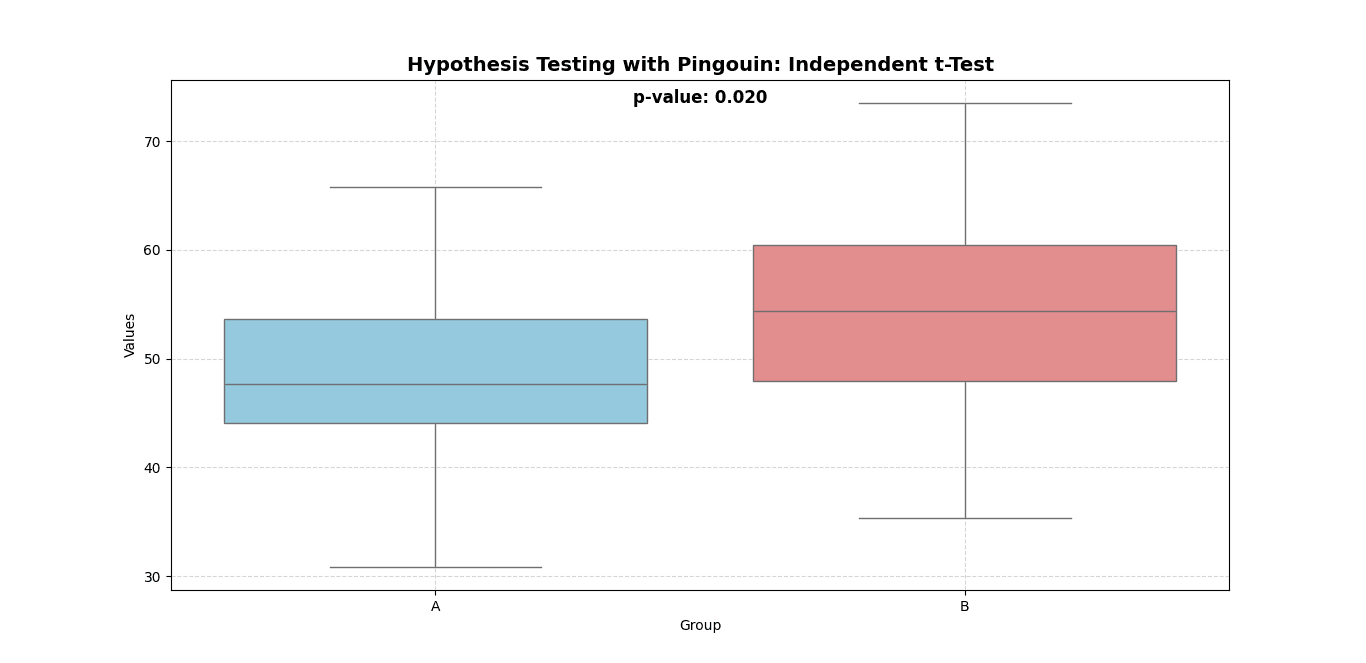
Performing a T-Test with Pingouin
A T-test checks whether the averages of two groups are different.
📌 Example: Let’s say we are testing if a new pain relief treatment works better than a placebo (fake treatment).
Here’s how we can do this in Pingouin:
import pingouin as pg
import pandas as pd

# Create sample data
data = {
    "Group": ["Control"] * 5 + ["Treatment"] * 5,  # Two groups
    "Pain_Threshold": [2.1, 2.3, 1.8, 2.5, 2.2, 3.0, 2.8, 3.1, 2.9, 3.2]  # Pain tolerance scores
}

df = pd.DataFrame(data)

# Run an independent T-test
ttest = pg.ttest(x=df[df["Group"] == "Control"]["Pain_Threshold"],
                 y=df[df["Group"] == "Treatment"]["Pain_Threshold"])

print(ttest)
Breaking Down the Output
When we run this, Pingouin gives us a table with these values:
| T | dof | alternative | p-val | CI95% | cohen-d | BF10 | power |
|---|---|---|---|---|---|---|---|
| -4.12 | 8 | two-sided | 0.003 | […] | 2.02 | 23.5 | 0.92 |
✔ T-value: Measures how different the two groups are. A larger T means a bigger difference.
✔ p-value: If it’s below 0.05, the difference is statistically significant. Here, 0.003 is much smaller than 0.05, so we reject the null hypothesis.
✔ Cohen’s d: This measures effect size (how strong the difference is). If d > 0.8, the effect is strong. Here, 2.02 is a very large effect.
✔ BF10 (Bayes Factor): If BF > 3, there’s strong evidence for a difference. Here, 23.5 is very strong evidence.
✔ Power: A high power value (close to 1) means the test is reliable. Here, it’s 0.92, which is excellent.
Conclusion: The pain relief treatment works significantly better than the placebo!
When Should You Use Different Tests?
T-tests are great, but they only work when comparing two groups. What if you have three or more groups? You need ANOVA.
ANOVA: Comparing More Than Two Groups
If you’re testing multiple treatments, use an ANOVA test (Analysis of Variance).
📌 Example: You are testing three different pain relief treatments and want to know if any of them work better than the others.
anova = pg.anova(data=df, dv="Pain_Threshold", between="Group")
print(anova)
✔ ANOVA checks for differences among three or more groups in one step, instead of doing multiple T-tests.
Bayesian Analysis: A Smarter Way to Test Hypotheses
Traditional hypothesis testing only tells us yes or no—whether a difference exists. But Bayesian analysis goes further: it tells us how likely one result is compared to another.
In Pingouin, we can calculate the Bayes Factor (BF), which shows how strong the evidence is.
bayes_ttest = pg.bayesfactor_ttest(x=df[df["Group"] == "Control"]["Pain_Threshold"],
                                   y=df[df["Group"] == "Treatment"]["Pain_Threshold"])
print(bayes_ttest)
✔ If BF > 3, there is strong evidence for a difference.
✔ If BF < 1/3, there is strong evidence against a difference.

Time Series Analysis: Finding Patterns Over Time
If your data is changing over time, you need time series analysis.
Example: A company wants to know if sales are increasing each month.
import numpy as np

# Generate random sales data
sales = np.random.randn(100)

# Check if past sales predict future sales
pg.autocorr(sales, lag=1)
✔ Autocorrelation checks if past values affect future values. If the result is high, past sales are influencing future sales.
Survival Analysis: Predicting When Events Will Happen
Survival analysis helps in fields like medicine (predicting patient survival) or engineering (predicting machine failures).
Example: Predicting when patients will recover based on their treatment.
df["Event"] = [1, 1, 0, 1, 0, 1, 1, 1, 0, 1]  # 1 = Recovery happened, 0 = No recovery
pg.coxph(data=df, duration="Pain_Threshold", event="Event")
✔ Cox regression helps us estimate how different factors affect survival times.
Tips for Using Pingouin Efficiently
- Always check for missing data before running tests.
- Use Bayesian analysis when you need stronger evidence.
- T-tests are great for comparing two groups, but use ANOVA for more.
- Time series analysis helps predict future trends based on past data.
- Survival analysis is useful in medicine, finance, and engineering.
Pingouin is one of the best Python libraries for statistical analysis because it makes hypothesis testing, Bayesian analysis, time series forecasting, and survival analysis incredibly simple.
If you want to do statistical testing without complex formulas, Pingouin is a must-have!
ArviZ – The Best Tool for Bayesian Statistical Analysis
Why Do We Need ArviZ?
When working with Bayesian statistics, we don’t just want a single answer—we want a range of possible values along with their probabilities. This is where ArviZ shines.
Most people use NumPy, pandas, and SciPy for general statistics, but Bayesian analysis needs a specialized tool. ArviZ is one of the best Python libraries for statistical analysis because it:
- Simplifies Bayesian analysis – No need to manually process complex probability distributions
- Works with PyMC, Stan, and NumPyro – These are popular tools for Bayesian modeling
- Creates visualizations – Helps you understand uncertainty in data
- Compares different Bayesian models – Makes it easier to choose the best model
If you’ve ever struggled with making sense of Bayesian model outputs, ArviZ is the solution.
1. Understanding Bayesian Analysis in Simple Terms
Before using ArviZ, let’s break down Bayesian statistics into simple steps.
In regular (frequentist) statistics, we use fixed probabilities.
In Bayesian statistics, we update our beliefs as new data arrives.
Example: Medical Diagnosis
Let’s say a doctor is diagnosing a patient for flu.
- The doctor starts with an initial belief:
- 50% chance the patient has the flu.
- The patient coughs a lot (new data).
- Flu patients often cough.
- The doctor updates the probability to 80% flu.
This process of updating beliefs with new data is called Bayesian inference.
Now, let’s see how ArviZ helps in practical Bayesian analysis.
2. Installing ArviZ
ArviZ is not included by default in Python, so you need to install it first:
pip install arviz
If you use PyMC, Stan, or NumPyro for Bayesian modeling, ArviZ will work perfectly with them.
3. Using ArviZ for Bayesian Analysis – Step by Step
Now, let’s go step by step through ArviZ’s key features.
Step 1: Loading Bayesian Model Data
To work with Bayesian models, we first need data. ArviZ provides example datasets so we can practice.
import arviz as az

# Load example Bayesian model results
data = az.load_arviz_data("centered_eight")

# Print the data structure
print(data)
This loads a sample Bayesian model, which we will use in later steps.
Step 2: Summarizing Bayesian Model Results
Once a Bayesian model is trained, we need to summarize the key statistics. Instead of manually calculating values, ArviZ provides a summary function:
summary = az.summary(data)
print(summary)
✔ What does this show?
- Mean – The average estimated value for each parameter
- Standard deviation – How much the values vary
- R-hat value – A measure of convergence (should be close to 1.0)
- Effective Sample Size (ESS) – A higher value is better
Tip: If the R-hat value is far from 1.0, the model hasn’t converged properly. You may need more data or better sampling methods.
Step 3: Visualizing Bayesian Probability Distributions
Since Bayesian models don’t give a single value but a range of probable values, visualization is crucial.
1. Posterior Distribution (Most Likely Values)
This shows where the most probable values lie:
az.plot_posterior(data, var_names=["mu"])
Tip: If the distribution is too wide, your model might need more data.
2. Trace Plot (Checking Model Stability)
A trace plot shows how the sampled values change over time.
az.plot_trace(data, var_names=["mu"])
Tip: If the lines look smooth and random, your model is stable. If they look like straight lines, your model might be stuck.
3. Pair Plot (Checking Parameter Relationships)
A pair plot shows how different parameters are related.
az.plot_pair(data, var_names=["mu", "tau"])
Tip: If parameters are highly correlated, the model might need adjustments.

Step 4: Comparing Bayesian Models
When working with Bayesian statistics, you often create multiple models and need to pick the best one.
1. WAIC (Widely Applicable Information Criterion)
WAIC tells us how well a model fits the data.
waic_results = az.waic(data)
print(waic_results)
Tip: Lower WAIC values mean a better model.
2. LOO (Leave-One-Out Cross-Validation)
LOO helps check if the model predicts new data accurately.
loo_results = az.loo(data)
print(loo_results)
Tip: If LOO is high, your model might be overfitting (fitting too closely to the training data).
Step 5: Checking Model Predictions
Once we have a Bayesian model, we need to verify if it predicts data correctly.
az.plot_ppc(data)
Tip: If predictions match real data, the model is good. If not, the model may need better priors or more data.
When Should You Use ArviZ?
ArviZ is useful for:
- Summarizing Bayesian models without manual calculations
- Visualizing probability distributions to understand uncertainty
- Comparing models to choose the best one
- Checking model predictions before making decisions
It works great for finance, AI, healthcare, marketing, and research where probability-based decisions matter.
Common Issues & Troubleshooting Tips
1. R-hat value is far from 1.0! What should I do?
✔ Run the model for more iterations or check if priors are too restrictive.
2. My trace plot looks like a straight line!
✔ Solution: The model might be stuck. Try a different sampler or adjust hyperparameters.
3. My posterior distribution is too wide!
✔ Solution: This means high uncertainty. You might need more data or better priors.
ArviZ is one of the best Python libraries for statistical analysis, but many people don’t use it.
- Makes Bayesian statistics easier
- It provides clear visualizations
- It helps compare different models
If you use Bayesian analysis, hypothesis testing, or statistical modeling, ArviZ is a tool you must use!
Must Read
- PyTorch Debugging Checklist: A Systematic Framework to Fix Models That Won’t Learn
- Why sorted() Is Safer Than list.sort() in Production Python Systems
- Monotonic Sequence in Python: 7 Practical Methods With Edge Cases, Interview Tips, and Performance Analysis
- How to Check if Dictionary Values Are Sorted in Python
- Check If a Tuple Is Sorted in Python — 5 Methods Explained
Lifelines – Survival Analysis in Python
What is Survival Analysis?
Survival analysis helps us predict the time until an event happens. This event could be:
- A customer canceling a subscription (churn analysis)
- A machine breaking down (failure prediction)
- A patient recovering or relapsing (medical research)
Instead of just saying “yes” or “no,” survival analysis focuses on “when” something will happen.
One of the best Python libraries for statistical analysis in this area is Lifelines. It provides simple tools to analyze and visualize survival data.
1. Installing Lifelines
First, install Lifelines using pip:
pip install lifelines
2. Understanding Survival Data
Before we start coding, let’s break down survival data:
Duration – How long a subject was observed (e.g., how many months a customer stayed subscribed)
🔹 Event Occurred? – Whether the event happened (e.g., whether the customer churned)
Here’s an example of survival data:
| Customer ID | Subscription Length (Months) | Churned? |
|---|---|---|
| 1 | 6 | Yes |
| 2 | 12 | No |
| 3 | 3 | Yes |
| 4 | 15 | No |
Let’s analyze this using Lifelines!
3. Kaplan-Meier Survival Curve
The Kaplan-Meier Estimator helps us visualize the probability of survival over time.
Step 1: Load Data
import pandas as pd
from lifelines import KaplanMeierFitter

# Create sample data
data = pd.DataFrame({
    "subscription_length": [6, 12, 3, 15, 10, 8, 20, 4, 5, 16],
    "churned": [1, 0, 1, 0, 1, 1, 0, 1, 1, 0]  # 1 = Churned, 0 = Still active
})

# Create a Kaplan-Meier model
kmf = KaplanMeierFitter()

# Fit the model
kmf.fit(data["subscription_length"], event_observed=data["churned"])

# Plot the survival curve
kmf.plot_survival_function()
✔ What does this curve show?
- The y-axis represents the probability of survival
- The x-axis represents time
- The curve drops as more customers churn
Tip: A steep drop means high churn risk at that time.
4. Cox Proportional Hazards Model
The Cox model helps us find what factors affect survival. For example, do higher prices lead to faster churn?
Step 1: Add More Data Features
from lifelines import CoxPHFitter

# Create dataset with additional features
data = pd.DataFrame({
    "subscription_length": [6, 12, 3, 15, 10, 8, 20, 4, 5, 16],
    "churned": [1, 0, 1, 0, 1, 1, 0, 1, 1, 0],
    "monthly_fee": [10, 15, 8, 20, 12, 9, 25, 7, 10, 22],  # Monthly fee in dollars
})

# Fit Cox model
cph = CoxPHFitter()
cph.fit(data, duration_col="subscription_length", event_col="churned")

# Show the model summary
cph.print_summary()
✔ What does this show?
- Positive coefficients mean higher risk of churn
- Negative coefficients mean longer survival
Tip: If higher prices lead to more churn, consider offering discounts or longer-term plans.
5. Predicting Survival for New Customers
Once we build a model, we can predict survival for new users.
# Predict survival for a new customer with a $12 monthly fee
new_customer = pd.DataFrame({"monthly_fee": [12]})
cph.predict_survival_function(new_customer).plot()
✔ This graph shows how long this customer is expected to stay.
6. When Should You Use Lifelines?
Lifelines is perfect for:
- Predicting customer churn in business
- Medical research (patient survival rates)
- Predicting equipment failure (preventive maintenance)
7. Common Issues & Troubleshooting
🔹 My survival curve drops too fast!
✔ Your customers might be churning quickly. Consider improving retention strategies.
🔹 The Cox model shows weird results!
✔ Check for high correlation between variables. Too many similar features can cause issues.
Lifelines is one of the best Python libraries for statistical analysis, yet many people don’t use it.
- Makes survival analysis simple
- It works great for business, healthcare, and engineering
- It helps you predict when things will happen
If you’re working with time-to-event data, Lifelines is a tool you must try!
sktime – A Hidden Gem for Time Series Analysis
When analyzing statistical data, most people focus on static datasets. But what if the data changes over time? sktime is a Python library designed specifically for time series analysis, making it one of the best Python libraries for statistical analysis. Unlike traditional tools like pandas and scikit-learn, sktime provides specialized models and utilities for handling time-dependent data.
Why Use sktime for Time Series Analysis?
Many people rely on pandas, NumPy, or scikit-learn for data analysis, but these libraries aren’t built for time-dependent data. sktime fills this gap by providing:
- Forecasting models (e.g., ARIMA, Exponential Smoothing, AutoARIMA)
- Time series classification (e.g., identifying patterns in stock prices)
- Time series regression (e.g., predicting future values based on past trends)
- Anomaly detection (e.g., spotting fraud in transaction data)
- Feature engineering (e.g., extracting useful information from time series)
With sktime, you don’t have to write complex custom functions for time-based analysis—it has everything built-in!
1. Installing sktime
To use sktime, install it with pip:
pip install sktime
pip install scikit-learn  # Needed for certain models
This installs sktime along with dependencies like NumPy and SciPy.
2. Time Series Forecasting with sktime
One of the most powerful features of sktime is forecasting, which helps predict future values based on historical data.
Step 1: Load Time Series Data
Let’s create some example data representing daily sales for a store:
import pandas as pd
from sktime.forecasting.model_selection import temporal_train_test_split

# Create a time series dataset
data = pd.Series(
    [100, 120, 130, 145, 160, 175, 180, 195, 205, 220,
     230, 245, 260, 275, 290, 305, 320, 335, 350, 370],
    index=pd.date_range(start="2024-01-01", periods=20, freq="D")
)

# Split into training and test sets
y_train, y_test = temporal_train_test_split(data, test_size=5)
- The dataset contains daily sales values from January 1, 2024.
- We split the data into a training set (first 15 days) and a test set (last 5 days).
Step 2: Train a Forecasting Model
Now, let’s train an AutoARIMA model, which automatically selects the best parameters for time series forecasting.
from sktime.forecasting.arima import AutoARIMA

# Train an AutoARIMA model
model = AutoARIMA(sp=7)  # Weekly seasonality (7 days)
model.fit(y_train)
- AutoARIMA adjusts itself based on the data’s patterns.
- The
sp=7parameter tells it to account for weekly trends.
Step 3: Make Predictions
Now, let’s predict future sales:
from sktime.forecasting.base import ForecastingHorizon

# Define future dates for prediction
fh = ForecastingHorizon(y_test.index, is_relative=False)

# Make predictions
y_pred = model.predict(fh)

print(y_pred)
- sktime forecasts sales for the next 5 days.
ForecastingHorizonensures predictions match future timestamps.
Tip: Adjust sp=12 for monthly seasonality or sp=365 for yearly trends.

3. Time Series Classification
Sometimes, we need to classify patterns in time series data. For example:
- Whether the stock going up or down?
- Is a patient’s heartbeat normal or irregular?
- Is an email spam or not, based on timing patterns?
sktime has built-in time series classification models, like Time Series Forest Classifier (TSF).
Step 1: Create Sample Data
from sklearn.model_selection import train_test_split
from sktime.classification.interval_based import TimeSeriesForestClassifier

# Example dataset
X = pd.DataFrame({
    "feature1": [100, 200, 150, 300, 250, 400, 500, 450, 600, 700],
    "feature2": [5, 10, 7, 15, 12, 18, 20, 22, 25, 30]
})
y = ["low", "high", "low", "high", "low", "high", "high", "low", "high", "low"]

# Split into training and test sets
X_train, X_test, y_train, y_test = train_test_split(X, y, test_size=0.3, random_state=42)
- Each row represents a time-dependent observation.
- The goal is to classify patterns based on previous data.
Step 2: Train a Classifier
# Train Time Series Forest Classifier
clf = TimeSeriesForestClassifier()
clf.fit(X_train, y_train)

# Make predictions
predictions = clf.predict(X_test)

print(predictions)
- sktime learns time-based patterns and predicts future labels.
- Works similarly to random forests but designed for time series.
Tip: Try k-nearest neighbors (KNN) or gradient boosting for different results.
4. Detecting Anomalies in Time Series Data
Anomalies in time series data indicate unusual behavior. Examples:
- Fraudulent transactions in banking
- Machine failures in industrial equipment
- Sudden spikes in website traffic
Step 1: Use Hampel Filter to Detect Anomalies
from sktime.transformations.series.outlier_detection import HampelFilter

# Initialize Hampel Filter
hampel = HampelFilter(window_length=5)

# Detect anomalies
outliers = hampel.fit_transform(data)

print(outliers)
- The Hampel Filter detects sudden spikes or dips.
- Useful for detecting errors or unexpected events.
Tip: Adjust window_length for more/less sensitivity.
5. Comparing sktime with Other Libraries
| Feature | sktime | statsmodels | scikit-learn | pandas |
|---|---|---|---|---|
| Time Series Forecasting | ✅ | ✅ | ❌ | ❌ |
| Anomaly Detection | ✅ | ❌ | ❌ | ❌ |
| Time Series Classification | ✅ | ❌ | ❌ | ❌ |
| Handles missing data | ✅ | ❌ | ❌ | ❌ |
| Feature Engineering | ✅ | ❌ | ❌ | ❌ |
✔ Why sktime?
- Easier than statsmodels for forecasting
- More powerful than pandas for time-based data
- Better than scikit-learn for time series classification
sktime is one of the best Python libraries for statistical analysis, especially for time series data.
- Handles forecasting, classification, and anomaly detection
- Works with scikit-learn, so it’s easy to use
- Simplifies time series problems that pandas & NumPy struggle with
If you work with time series data, sktime is a must-have tool!
PyJanitor – Clean Data Before Statistical Analysis
Before running any statistical analysis, data cleaning is a must. Messy data can lead to wrong conclusions, inaccurate models, and wasted time. This is where PyJanitor shines.
PyJanitor is a hidden gem in the Python ecosystem, designed to simplify data cleaning, preprocessing, and feature engineering. It extends pandas with extra functions, making it easier to remove duplicates, fix missing values, rename columns, and clean messy datasets.
If you’re working with large datasets, PyJanitor helps reduce manual effort and speeds up your workflow. That’s why it’s one of the best Python libraries for statistical analysis.
Why Use PyJanitor?
Most data cleaning tasks require writing custom functions with pandas. PyJanitor provides built-in functions that:
- Remove missing values quickly
- Rename columns easily without using complex dictionaries
- Filter and transform data in a single step
- Detect and remove duplicate rows
- Handle categorical data efficiently
With PyJanitor, you write less code and make your data ready for statistical modeling and hypothesis testing faster.
1. Installing PyJanitor
Before using PyJanitor, install it with pip:
pip install pyjanitor
It works on top of pandas, so you don’t need to change your workflow.
2. Quick Data Cleaning with PyJanitor
Let’s start with a messy dataset and clean it up using PyJanitor.
Step 1: Create a Messy Dataset
import pandas as pd

# Creating a messy dataset
data = pd.DataFrame({
    "Column 1": [" Alice ", "Bob", "Charlie", None, "David"],
    "age(years)": [25, 30, None, 45, 35],
    "Income($)": [50000, 60000, 55000, None, 70000],
    "gender": ["Female", "Male", "Male", "Male", None]
})

print(data)
| Column 1 | age(years) | Income($) | gender |
|---|---|---|---|
| Alice | 25 | 50000 | Female |
| Bob | 30 | 60000 | Male |
| Charlie | None | 55000 | Male |
| None | 45 | None | Male |
| David | 35 | 70000 | None |
🚨 Problems in the dataset:
- Extra spaces in names
- Messy column names
- Missing values
- Inconsistent capitalization
Step 2: Clean the Data with PyJanitor
import janitor

# Cleaning the dataset
cleaned_data = (
    data
    .clean_names()  # Standardize column names
    .dropna()  # Remove rows with missing values
    .strip_strings()  # Remove extra spaces from text
    .fill_empty("gender", "Unknown")  # Replace empty values
)

print(cleaned_data)
| column_1 | age_years | income_dollar | gender |
|---|---|---|---|
| Alice | 25 | 50000 | Female |
| Bob | 30 | 60000 | Male |
✔ What PyJanitor did:
- Standardized column names (removed spaces and symbols)
- Dropped rows with missing values
- Removed extra spaces from names
- Replaced empty gender values with “Unknown”
Tip: If you want to replace missing values instead of dropping them, use .fillna().
3. Handling Duplicate Data
Duplicate data can skew statistical analysis. Let’s fix it with PyJanitor.
data = pd.DataFrame({
    "name": ["Alice", "Bob", "Charlie", "Alice"],
    "age": [25, 30, 35, 25],
    "income": [50000, 60000, 70000, 50000]
})

# Remove duplicate rows
cleaned_data = data.remove_duplicates()

print(cleaned_data)
✔ PyJanitor automatically removes duplicate rows with just one function!
4. Filtering and Selecting Data
When preparing data for statistical modeling, you may need to filter specific rows or select certain columns.
# Select rows where income is above 55,000
filtered_data = cleaned_data.filter_column("income", ">", 55000)

print(filtered_data)
✔ This keeps only the rows where income > 55,000, without needing pandas’ long query() function.
Tip: You can use ==, !=, <, >, <=, >= for filtering.
5. Feature Engineering for Statistical Analysis
Feature engineering is crucial for Bayesian analysis, survival analysis, and hypothesis testing. PyJanitor makes it easy!
Step 1: Add New Features
# Create a new column based on conditions
data = data.add_column("high_income", data["income"] > 55000)

print(data)
✔ Now, the dataset has a new “high_income” column showing True or False.
Step 2: Convert Categorical Data
Many statistical models need numeric input. Convert categorical data into numbers:
# Convert gender into numeric values
data = data.encode_categorical("gender")

print(data)
✔ This turns “Male” into 0 and “Female” into 1, making it ready for analysis.
6. Comparing PyJanitor with Other Libraries
| Feature | PyJanitor | pandas | NumPy | scikit-learn |
|---|---|---|---|---|
| Standardizing column names | ✅ | ❌ | ❌ | ❌ |
| Removing missing values | ✅ | ✅ | ❌ | ✅ |
| Detecting duplicates | ✅ | ✅ | ❌ | ✅ |
| Feature engineering | ✅ | ❌ | ❌ | ✅ |
| Filtering rows easily | ✅ | ❌ | ❌ | ❌ |
✔ Why PyJanitor?
- More powerful than pandas for cleaning data
- Works well with scikit-learn for machine learning
- Saves time on repetitive data preprocessing tasks
PyJanitor is one of the best Python libraries for statistical analysis because clean data leads to better models.
Why use PyJanitor?
- Speeds up data cleaning and preprocessing
- Works seamlessly with pandas
- Helps with feature engineering for Bayesian, survival, and time series analysis
Tip: If you’re doing hypothesis testing or machine learning, clean your data first with PyJanitor. It will save you hours of debugging later!
Patsy – Make Statistical Modeling Easy in Python
When working with statistics in Python, you often need to prepare data before using it in models. Usually, you have to manually clean data, transform variables, and handle categories.
This can be time-consuming and complicated. Patsy solves this problem by making it easy to prepare data for statistical models using simple formulas.
It is one of the best Python libraries for statistical analysis, especially for:
- Regression analysis
- Hypothesis testing
- Bayesian statistics
- Survival analysis
Let’s see how Patsy works with step-by-step examples.
1. Installing Patsy
Before using Patsy, install it with this command:
pip install patsy
Now, you can easily prepare your data for statistical models.
2. What Does Patsy Do?
Patsy simplifies data preparation for models. It helps with:
- Defining models using formulas (like in R)
- Automatically converting categorical data into numbers
- Creating interaction terms (when two factors affect the outcome together)
- Applying transformations (log, square, standardization)
Instead of manually writing code to prepare data, you can just write a formula like:
"salary ~ experience + education"
This tells Patsy:
- “Predict salary using experience and education as factors.”
- Patsy automatically converts data into a matrix ready for models.
3. Using Patsy to Prepare Data
Example: Converting Data into Model-Ready Format
import pandas as pd
import patsy

# Sample dataset
data = pd.DataFrame({
    "experience": [1, 3, 5, 7, 9],
    "salary": [30000, 40000, 50000, 60000, 70000]
})

# Create design matrices for regression
y, X = patsy.dmatrices("salary ~ experience", data)

print(X)
✔ What does this do?
- Converts “salary ~ experience” into numerical matrices
- Automatically adds an intercept (a column of ones for regression)
- Makes data ready for statsmodels or scikit-learn
Now, you don’t need to manually create feature matrices.
4. Handling Categorical Variables Automatically
Most datasets contain categorical variables (e.g., “High School”, “Bachelor”, “PhD”).
Machine learning models need numbers, not text.
Patsy automatically converts categories into dummy variables.
Example: Converting Categorical Variables
# Sample dataset with categorical education levels
data = pd.DataFrame({
    "education": ["High School", "Bachelor", "Master", "PhD", "Bachelor"],
    "salary": [30000, 40000, 50000, 60000, 70000]
})

# Convert categorical variable into dummy variables
y, X = patsy.dmatrices("salary ~ C(education)", data)

print(X)
✔ What does this do?
- C(education) tells Patsy to treat education as a category.
- It creates dummy variables for each education level.
- This helps models understand categories as numbers.
5. Creating Interaction Terms
Sometimes, two factors together affect the outcome.
For example, education and experience may both influence salary.
Patsy allows easy interaction terms using *.
Example: Interaction Between Experience and Education
# Sample dataset
data = pd.DataFrame({
    "experience": [1, 3, 5, 7, 9],
    "education": ["High School", "Bachelor", "Master", "PhD", "Bachelor"],
    "salary": [30000, 40000, 50000, 60000, 70000]
})

# Include interaction between experience and education
y, X = patsy.dmatrices("salary ~ experience * C(education)", data)

print(X)
✔ What does this do?
- The
*operator means “include experience, education, and their interaction.” - The model will see how education affects salary at different experience levels.
📌 Tip: Use : for only interaction and * for main effects + interaction.
6. Applying Transformations
Sometimes, you need to apply math functions to features before modeling.
Patsy lets you apply transformations inside the formula.
Example: Applying a Log Transformation
y, X = patsy.dmatrices("salary ~ np.log(experience)", data)
✔ This applies a logarithm to the experience column before running the model.
Other useful transformations:
- Standardization:
salary ~ scale(experience) - Polynomial features:
salary ~ experience + I(experience**2)
📌 Tip: Use I() to apply operations like squaring (x**2).
7. Using Patsy with Statsmodels
Patsy is designed to work with statsmodels, a popular library for statistical modeling.
Example: Running Linear Regression
import statsmodels.api as sm

# Create design matrices
y, X = patsy.dmatrices("salary ~ experience", data)

# Fit the regression model
model = sm.OLS(y, X).fit()

# Print summary
print(model.summary())
✔ What does this do?
- Uses Patsy to format the data
- Runs linear regression using statsmodels
- Automatically includes an intercept
Now, you don’t have to manually transform data before running models.
8. Why Use Patsy Instead of Pandas?
| Feature | Patsy | Pandas | Scikit-learn |
|---|---|---|---|
| Formula-based modeling | ✅ | ❌ | ❌ |
| Dummy encoding (categorical variables) | ✅ | ✅ | ✅ |
| Interaction terms | ✅ | ❌ | ✅ |
| Polynomial features & transformations | ✅ | ❌ | ✅ |
| Seamless integration with statsmodels | ✅ | ❌ | ❌ |
✔ Why Patsy?
- Easier than pandas for preparing model inputs
- More flexible than scikit-learn for feature engineering
- Saves time by automating transformations
Patsy is one of the best Python libraries for statistical analysis because it makes data preparation easy.
🚀 Why should you use Patsy?
- Converts formulas into ready-to-use matrices
- Handles categorical variables, interactions, and transformations
- Works perfectly with statsmodels and scikit-learn
Tip: If you’re doing regression analysis, Bayesian models, or hypothesis testing, use Patsy to save time and avoid manual data transformation!
Conclusion: Choosing the Right Library for Your Needs
When working with statistical analysis in Python, choosing the right library can save you time and effort. Each library has unique strengths, so the best choice depends on your specific needs.
- If you need Bayesian statistical analysis → Use ArviZ for easy diagnostics and visualization.
- When you’re working with survival analysis → Lifelines is the best tool for Kaplan-Meier and Cox models.
- For time series analysis → Sktime simplifies forecasting and machine learning for time-based data.
- If your data needs cleaning before analysis → PyJanitor automates repetitive tasks like removing duplicates and standardizing columns.
- If you want to prepare data for statistical models → Patsy makes it easy to handle categorical variables, transformations, and interactions.
Each of these hidden Python libraries is a powerful tool that can make your work easier.
Tip: If you’re working with complex data and models, combining these libraries with Statsmodels and Scikit-learn will give you even more flexibility.
Next Steps: Try out these libraries in your projects and see how they improve your workflow!
FAQs
What makes these Python libraries “hidden gems” for statistical analysis?
Can I use these libraries with pandas and NumPy?
Which library is best for predictive modeling?
How can I install and start using these libraries?
pip install arviz lifelines sktime pyjanitor patsyOnce installed, check the documentation and try running some example code to see how they fit into your workflow!


Leave a Reply