Confidence Interval in Data Science: A Complete Guide

Introduction to Confidence Intervals in Data Science

A confidence interval is a helpful way to estimate how close our predictions are to the actual values. Instead of giving just one number, it provides a range where the true value is likely to be. This makes predictions more useful and reliable.

With confidence intervals, we can say, “We are quite sure the real value is within this range,” instead of just guessing. This method helps us make decisions based on evidence, even when we have only a small amount of data.

In this post, I’ll explain confidence intervals in a simple way with real-life examples. You’ll learn how they work and how they can make your data analysis stronger. If you want to improve your data science skills, this is a great concept to learn. Stay tuned—it might become one of your favorite tools!

What is a Confidence Interval?

A confidence interval gives us a range of values where the true value is likely to be. Instead of just one number, it gives a better picture of how accurate our estimate is.

For example, if customer ratings average 4.2 stars, the confidence interval might say, “We are quite sure the real average is between 4.1 and 4.3 stars.”

This makes confidence intervals a useful tool for checking how reliable our predictions are.

Why Confidence Intervals are Important in Data Science

Confidence intervals are an important tool in data science. Here’s why they matter:

• Accuracy Check: They show us how precise our results are. Without them, we’re just making a prediction without knowing whether it is close to the reality.
• Better Decisions: By giving a range where the true values likely fall, they help us make smarter and more informed choices. They act as a safety net when working with data.
• Comparisons: Confidence intervals help when comparing groups, models, or methods. They show whether differences are real or just happened by chance.

In short, confidence intervals help us trust our analysis and avoid overconfident conclusions. They’re like a reality check for our numbers!

Applications of Confidence Intervals in Machine Learning and Data Science

Confidence intervals are everywhere in data science and machine learning:

• Model Evaluation: They give a range for metrics like accuracy or error rate, helping us see if a model’s results are trustworthy.
• A/B Testing: When testing two versions of a product or ad, confidence intervals show if one truly performs better or if the difference is just random chance.
• Predictive Analysis: They help us understand how reliable our predictions are, especially when working with small data samples or new models.

In short, confidence intervals bring clarity and confidence to data-driven decisions!

Understanding the Basics of Confidence Intervals

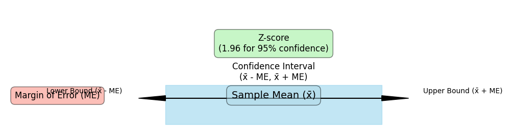
Components of a Confidence Interval

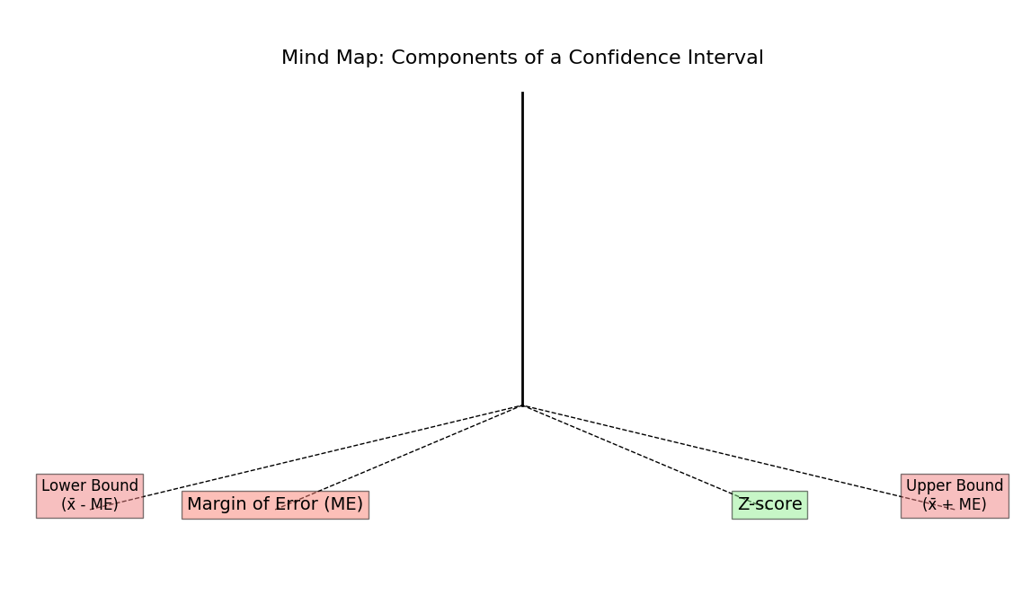
Here are the key parts of a confidence interval:

• Confidence Level: This tells us how sure we are about the interval. A 95% confidence level means we’re 95% certain the real value is within our range.
• Margin of Error: This shows how much our estimate could be off. A smaller margin means a more precise estimate, creating a tighter range.
• Point Estimate: This is the central value, like an average. The confidence interval is built around this best guess.

Each part helps make the interval more reliable and useful, adding clarity and confidence to our results.

Key Terminology in Confidence Intervals

Understanding a few basic terms makes confidence intervals easier to use:

• Population and Sample: The population is the entire group we’re interested in. But since we can’t always collect data from everyone, we use a sample—a smaller group that represents the whole. Confidence intervals help us estimate things about the entire population using just that sample.
• Statistical Significance and Confidence Intervals: If a confidence interval doesn’t include a certain value—like zero—it often means the result is statistically significant. This suggests our findings are real and not just random chance.

These ideas help us use confidence intervals the right way and trust our results!

How to Calculate Confidence Intervals in Data Science

There are several ways to calculate confidence intervals, and it doesn’t have to be complicated! Whether you use a simple formula, Python, or more advanced methods, the goal is the same—getting a reliable range for your estimates.

Here’s an overview of common methods, from traditional calculations to code-based approaches, so you can pick the best one for your analysis.

Traditional Formula-Based Methods

One of the most common ways to calculate a confidence interval is by using a basic formula. This involves the sample mean, sample size, and either a Z-score or T-score:

• Z-scores are used when we know the population standard deviation or have a large sample size.
• T-scores are used when the sample size is small or we don’t know the population standard deviation.

This formula-based method is simple and effective, making it a great starting point for confidence interval calculations.

Bootstrap Methods for Confidence Intervals

Bootstrap methods take a different approach by using resampling instead of a fixed formula. Here’s how they work:

• We create many “bootstrapped” samples by randomly sampling with replacement from our data.
• We calculate the mean (or another statistic) for each sample.
• The confidence interval is then based on the variability across these samples.

Bootstrap methods are popular because they’re flexible and don’t require strict assumptions about the data’s distribution. They work well even when traditional formulas aren’t ideal!

Using Python for Confidence Interval Calculations

Python makes it easy to calculate confidence intervals. You can use SciPy, NumPy, and Pandas.

• SciPy has built-in functions:
  • scipy.stats.norm.interval() for Z-scores.
  • scipy.stats.t.interval() for T-scores.
• NumPy helps with basic calculations:
  • Find the mean and standard deviation.
  • Work with arrays easily.
• Pandas is great for data tables:
  • Pick specific columns.
  • Filter rows and group data.

These tools help you calculate confidence intervals fast!

Python Code for Confidence Interval Calculation with SciPy and NumPy

If you’re ready to dive into the code, here’s a quick example using SciPy and NumPy. This code calculates a confidence interval for a sample mean.

import numpy as np
from scipy import stats

# Example data
data = [22, 25, 27, 28, 30, 31, 35, 36]

# Calculate mean and standard error
mean = np.mean(data)
std_error = stats.sem(data)  # Standard error of the mean

# Confidence interval with 95% confidence level
confidence_interval = stats.t.interval(0.95, len(data)-1, loc=mean, scale=std_error)

print("Mean:", mean)
print("Confidence Interval:", confidence_interval)

This code uses the T-score method, which is ideal for small sample sizes. SciPy handles the heavy lifting, and the results will give you a 95% confidence interval for the sample mean.

Calculating Confidence Intervals with Pandas

If your data is in a Pandas DataFrame, you can easily calculate confidence intervals for each column or group. Here’s an example:

import pandas as pd
from scipy import stats

# Example DataFrame
df = pd.DataFrame({
    'Group': ['A', 'A', 'A', 'B', 'B', 'B'],
    'Values': [23, 25, 27, 35, 37, 39]
})

# Calculate confidence interval for each group
def calculate_ci(series):
    mean = series.mean()
    std_error = stats.sem(series)
    interval = stats.t.interval(0.95, len(series)-1, loc=mean, scale=std_error)
    return interval

ci_by_group = df.groupby('Group')['Values'].apply(calculate_ci)
print(ci_by_group)

This approach makes it easy to calculate confidence intervals for multiple groups in one go.

Step-by-Step Guide to Confidence Interval Calculation

Let’s go through the process of calculating a confidence interval together.

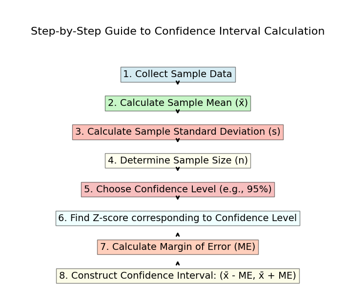
1. Determine the Sample Mean and Sample Standard Deviation

To calculate a confidence interval, start with these two key values:

• Sample Mean: The average of your sample data. Add up all the values and divide by the total number of data points.
• Sample Standard Deviation: This measures how spread out the data is. A higher value means more variability.

If you’re using Python, you can calculate these values quickly:

import numpy as np

# Sample data
data = [23, 25, 27, 29, 30, 31, 33]

# Calculate mean and standard deviation
sample_mean = np.mean(data)
sample_std_dev = np.std(data, ddof=1)  # ddof=1 for sample standard deviation

print("Sample Mean:", sample_mean)
print("Sample Standard Deviation:", sample_std_dev)

2. Choosing the Correct Confidence Level

Next, decide on your confidence level. Common levels are:

1. 90%: Used when you want to be fairly confident, but willing to allow a bit more error.
2. 95%: The most commonly used level, balancing confidence with precision.
3. 99%: Gives high confidence but results in a wider interval.

In most cases, a 95% confidence level is the go-to. This choice impacts the size of your interval: higher confidence means a larger range, while lower confidence means a smaller range.

3. Understanding Z and T Distributions in Calc ulations

Now that you have your sample mean and standard deviation, the next step is choosing between the Z distribution and T distribution:

• Use Z-scores if your sample is large (usually over 30) or you know the population standard deviation.
• Use T-scores if your sample is small (under 30) or the population standard deviation is unknown.

The T distribution is slightly wider, making it better for smaller samples because it adds a bit of cushion to your estimate.

Here’s how to calculate a 95% confidence interval using the T distribution in Python:

from scipy import stats

# Define confidence level
confidence_level = 0.95
degrees_freedom = len(data) - 1  # Degrees of freedom for T distribution
standard_error = sample_std_dev / np.sqrt(len(data))

# Calculate confidence interval
confidence_interval = stats.t.interval(confidence_level, degrees_freedom, loc=sample_mean, scale=standard_error)

print("Confidence Interval:", confidence_interval)

In this example, we use the scipy.stats.t.interval function, which handles the calculation using the T distribution.

Must Read

• How to Return Multiple Values from a Function in Python
• Parameter Passing Techniques in Python: A Complete Guide
• A Complete Guide to Python Function Arguments
• How to Create and Use Functions in Python
• Find All Divisors of a Number in Python

Different Types of Confidence Intervals in Data Science

Now, Let’s explore the different types of confidence intervals and see the math behind them.

1. Mean Confidence Interval

A mean confidence interval helps estimate the average value of a population based on sample data.

Mathematical Approach:

• Formula:

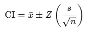
• xˉ = sample mean
• Z = Z-score corresponding to your confidence level
• s = sample standard deviation
• n = sample size

Python Example:

import numpy as np
from scipy import stats

# Sample data
data = [23, 25, 27, 29, 30, 31, 33]
sample_mean = np.mean(data)
sample_std_dev = np.std(data, ddof=1)
n = len(data)

# Z-score for 95% confidence
z_score = stats.norm.ppf(0.975)  
margin_of_error = z_score * (sample_std_dev / np.sqrt(n))

confidence_interval = (sample_mean - margin_of_error, sample_mean + margin_of_error)

print("Mean Confidence Interval:", confidence_interval)

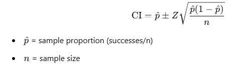
2. Proportion Confidence Interval

This interval is used when dealing with proportions, such as the percentage of respondents who favor a product.

Mathematical Approach:

• Formula

# Sample data
successes = 40  # e.g., number of people who like a product
n = 100         # total sample size
p_hat = successes / n  # sample proportion

# Z-score for 95% confidence
z_score = stats.norm.ppf(0.975)

# Margin of error
margin_error = z_score * np.sqrt((p_hat * (1 - p_hat)) / n)
confidence_interval_proportion = (p_hat - margin_error, p_hat + margin_error)

print("Proportion Confidence Interval:", confidence_interval_proportion)

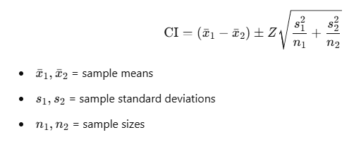
3. Difference of Means Confidence Interval

This interval helps compare the means of two different groups to see if there’s a significant difference.

Mathematical Approach:

• Formula:

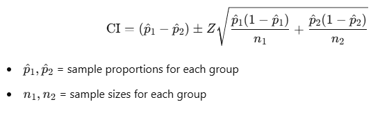
4. Difference of Proportions Confidence Interval

This interval compares the proportions from two groups.

Mathematical Approach:

• Formula:

5. Confidence Intervals for Regression Analysis

In regression, confidence intervals can be calculated for predicted values to understand the uncertainty around predictions.

Mathematical Approach:

• Formula for a predicted value’s confidence interval: CI=y^±t⋅SEy^
  • y^​ = predicted value from the regression model
  • t = t-score based on confidence level and degrees of freedom
  • SEy^​​ = standard error of the predicted value

Python Example:

import pandas as pd
import statsmodels.api as sm

# Sample data
data = pd.DataFrame({
    'X': [1, 2, 3, 4, 5],
    'Y': [2, 3, 5, 7, 11]
})

# Fit a linear regression model
X = sm.add_constant(data['X'])  # Add constant for intercept
model = sm.OLS(data['Y'], X).fit()

# Get predictions and confidence intervals
predictions = model.get_prediction(X)
pred_int = predictions.summary_frame(alpha=0.05)  # 95% confidence interval

print(pred_int[['mean', 'mean_ci_lower', 'mean_ci_upper']])

Choosing the Right Type of Confidence Interval

In data science, choosing the right type of confidence interval is crucial because different types of data need different approaches.

Here are the two main types:

• Mean Confidence Interval: Used when estimating the average value of a population from a sample. This is common when working with numerical data, like test scores or product prices.
• Proportion Confidence Interval: Used when dealing with categorical data, like survey results or customer preferences. It helps estimate what percentage of a population falls into a certain category.

Each type ensures that your estimates are accurate and realistic, helping you make informed decisions based on data!

When to Use a Mean Confidence Interval vs. a Proportion Confidence Interval

A mean confidence interval is useful when:

• Your data is numerical (e.g., heights, weights, test scores).
• You have a sample and want to estimate the average for a larger population.

Example:

Suppose you want to estimate the average test score of students in a school. Instead of surveying every student, you take a sample of 50 students and calculate their mean score. A mean confidence interval helps you express how confident you are that the true school-wide average falls within a certain range.

Mathematical Context:

If you have numerical data and want to estimate the average while accounting for uncertainty, a mean confidence interval is the right choice. It provides a range that is likely to contain the true mean, rather than relying on a single estimate

Formula Recap:

When to Use Proportion Confidence Interval:

• Your data involves counts or percentages (e.g., survey responses, success rates).
• You want to estimate the likelihood of an event happening based on a sample.

Example:

Imagine you conduct a survey asking 1,000 people whether they prefer Brand A over Brand B. If 600 people say yes, you might want to estimate what percentage of the entire population prefers Brand A. A proportion confidence interval helps you express how confident you are in this percentage.

Mathematical Context:

If you’re working with yes/no, success/failure, or category-based data, a proportion confidence interval allows you to estimate the true percentage in the population while accounting for sampling variability.

Formula Recap

Selecting the Correct Type for Different Data Science Applications

When deciding which confidence interval to use, consider the type of data you’re working with.

Mean Confidence Intervals

Use when your data is numerical (averages, measurements).

Applications:

• Analyzing average performance metrics (e.g., average sales per month).
• Comparing average values between groups (e.g., average income across regions).

Example:

A company wants to know the average time customers spend on their website. They take a sample of visits and calculate a mean confidence interval to estimate the true average for all users.

• Analyzing average performance metrics (e.g., average sales per month).
• Comparing average values between different groups (e.g., average income between regions).

Proportion Confidence Intervals

Use when your data is categorical (percentages, success/failure rates).

Applications:

• Evaluating survey data to determine public opinion.
• Analyzing success rates (e.g., conversion rates in marketing).

Example:

A restaurant conducts a survey asking customers if they enjoyed their meal. They calculate a proportion confidence interval to estimate the percentage of customers with a positive experience.

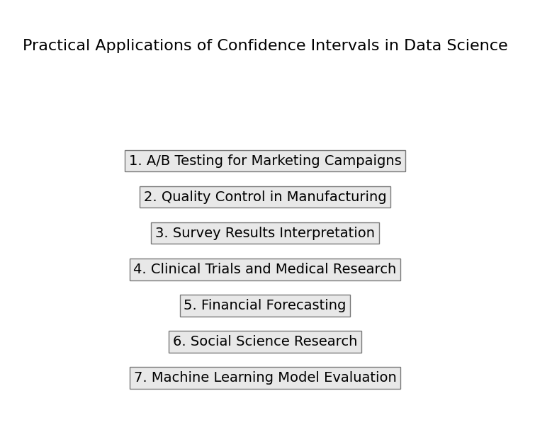
Practical Applications of Confidence Intervals in Data Science

Confidence intervals are more than just numbers. They help you make decisions based on data, whether in A/B testing, evaluating model accuracy, or comparing machine learning models.

Confidence Intervals in A/B Testing

A/B testing is widely used in marketing and product design. You compare two versions of something—like a webpage—to see which one performs better. Here’s how confidence intervals play a role.

Mathematical Perspective:

• When you collect data from your A/B test, you typically look at proportions or means.
• Let’s say you have the following results for two landing pages:
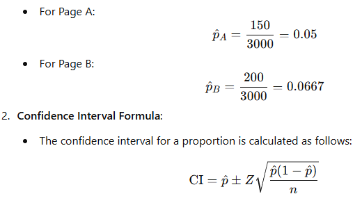
  • Page A: 150 conversions out of 3,000 visitors.
  • Page B: 200 conversions out of 3,000 visitors.

Calculating Confidence Intervals:

1. Proportion Calculation:

3. Python Implementation: You can use Python to calculate this. Here’s a snippet using scipy:

import numpy as np
from scipy import stats

# Data for Page A
conversions_A = 150
visitors_A = 3000
p_A = conversions_A / visitors_A

# Data for Page B
conversions_B = 200
visitors_B = 3000
p_B = conversions_B / visitors_B

# Calculate confidence intervals
def calculate_ci(p, n, confidence=0.95):
    z = stats.norm.ppf((1 + confidence) / 2)
    ci = z * np.sqrt((p * (1 - p)) / n)
    return (p - ci, p + ci)

ci_A = calculate_ci(p_A, visitors_A)
ci_B = calculate_ci(p_B, visitors_B)

print(f"Confidence Interval for Page A: {ci_A}")
print(f"Confidence Interval for Page B: {ci_B}")

Evaluating Model Accuracy and Predictions with Confidence Intervals

When you create models, it’s important to know how accurate they are. Confidence intervals can help you understand the uncertainty in your predictions.

Mathematical Perspective:

• Suppose you have a regression model that predicts house prices based on various features. You want to estimate how accurate your predictions are.

1. Mean Prediction and Confidence Interval:
   • Say your model predicts a house price of $300,000, and you have the following information from your sample:
   • mean (yˉ​): $300,000
   • Sample standard deviation (s): $50,000
   • Sample size (nnn): 30
2. Confidence Interval Calculation:

Here, t is the t-score corresponding to your desired confidence level.

3. Python Code Example:

from scipy import stats

# Sample data
mean_prediction = 300000
sample_std_dev = 50000
sample_size = 30

# Calculate t-score for 95% confidence
t_score = stats.t.ppf(0.975, df=sample_size - 1)

# Calculate the confidence interval
margin_of_error = t_score * (sample_std_dev / np.sqrt(sample_size))
ci_price = (mean_prediction - margin_of_error, mean_prediction + margin_of_error)

print(f"Confidence Interval for house price prediction: {ci_price}")

Using Confidence Intervals in Machine Learning for Model Comparison

When working with different models, you want to know which one is better. Confidence intervals can help you compare them effectively.

Mathematical Perspective:

• You may have two models predicting a specific outcome, and you want to see if their performance metrics (like RMSE) are significantly different.

1. Calculating RMSE:
   • For Model A, let’s say you calculated an RMSE of 1.5 with a confidence interval of (1.2, 1.8).
   • For Model B, the RMSE is 1.2 with a confidence interval of (0.9, 1.5).
2. Comparison:
   • By examining these intervals, you can see if there is an overlap. If they don’t overlap, one model is likely performing better than the other.
3. Python Implementation: Here’s how you could visualize this in Python using matplotlib:

import matplotlib.pyplot as plt

# RMSE values and confidence intervals
models = ['Model A', 'Model B']
rmse_values = [1.5, 1.2]
lower_bounds = [1.2, 0.9]
upper_bounds = [1.8, 1.5]

# Plotting
plt.bar(models, rmse_values, yerr=[np.array(rmse_values) - np.array(lower_bounds), 
                                     np.array(upper_bounds) - np.array(rmse_values)], capsize=5)
plt.ylabel('RMSE')
plt.title('Model Comparison with Confidence Intervals')
plt.show()

Interpreting Confidence Intervals: Avoiding Common Mistakes

How to Interpret Confidence Intervals Correctly

Interpreting confidence intervals can seem tricky, but don’t worry! Let’s break it down step by step.

We’ll cover:

• What a 95% confidence interval really means
• Common mistakes people make
• Pitfalls to avoid

Understanding confidence intervals helps you make better decisions based on data.

What a 95% Confidence Interval Actually Means

When you hear “95% confidence interval,” it might sound complicated, but it’s really just a way to express uncertainty in a clear and structured way.

What It Really Means:

If we took many samples from a population and calculated a confidence interval for each one, about 95% of those intervals would contain the true population value (like an average or proportion).

So, if we say we have a 95% confidence interval for the average height of a group, we’re saying we’re pretty sure (95% sure!) that the true average lies within that range.

Example:

Let’s say you survey people about their weekly spending and find a 95% confidence interval of $50 to $70. This means:

“I am 95% confident that the true average spending of the population is between $50 and $70.”

Confidence intervals help us make better decisions by giving us a realistic range instead of just a single guess!

Common Misinterpretations and Misuses of Confidence Intervals

1. Thinking the true value is “inside” the interval with 95% certainty

• Wrong idea: If we get a confidence interval of (4.1, 4.3), some people think, “There is a 95% chance that the true value is in this range.”
• The truth: Once the interval is calculated, it’s fixed. Instead, the correct way to think about it is: if we repeated this process many times, about 95% of those intervals would contain the true value.

Example: Imagine you’re shooting arrows at a target. If your method is 95% accurate, it doesn’t mean a single shot is 95% inside the bullseye—it means that over many shots, you’ll hit it 95% of the time.

2. Thinking a narrow interval always means better accuracy

• Wrong idea: If the confidence interval is very small, some assume it must be highly accurate.
• The truth: A narrow interval can be misleading if it’s based on a small sample size that doesn’t represent the full population.

Example: If you ask only five people about their height, the range might be small, but it doesn’t reflect everyone’s height. Asking 500 people gives a much more trustworthy estimate.

3. Using confidence intervals on the wrong data

• Wrong idea: Confidence intervals work for everything in data analysis.
• The truth: They only work when the data meets certain conditions, like following a normal distribution or having enough samples.

Example: If you try using confidence intervals on random social media trends, where data changes unpredictably, the results might not be useful.

Key Takeaway:

Confidence intervals are powerful, but they must be used correctly. It’s like measuring with a ruler—if the ruler is bent or used on the wrong object, the measurement won’t be reliable!

Pitfalls to Avoid with Confidence Intervals

Understanding these mistakes will help you make better data-driven decisions!

Overconfidence in Small Sample Sizes

Using a small sample size can lead to misleading confidence intervals.

• Lack of Representation: A small sample might not include enough variety from the full population. This can make your interval too narrow or too wide, meaning it doesn’t truly reflect reality.

Example: Suppose you want to estimate the average weight of apples in a large orchard. If you only weigh five apples, your confidence interval might be very small, making it look precise. But in reality, it could be far from the true average because you haven’t accounted for all apple varieties!

A larger sample size gives a more reliable and realistic confidence interval.

Ignoring the Importance of Confidence Levels

Picking the right confidence level affects how useful your interval is. Here’s what to keep in mind:

Confidence Level Impact

• A 95% confidence interval is common, but it’s not always the best choice for every situation.
• Higher confidence levels (like 99%) create wider intervals, making them more cautious but also less precise.
• Lower confidence levels (like 90%) create narrower intervals, giving a more specific estimate but with less certainty.

Understanding Trade-offs

• If certainty is critical, go for a higher confidence level (like 99%). Example: Medical research, where accuracy is crucial.
• If speed and practicality matter, a lower confidence level (like 90%) might be enough. Example: Quick business forecasts, where you just need a general idea.

It’s all about balancing precision and confidence based on your needs!

Advanced Confidence Interval Techniques for Data Scientists

Once you understand the basics, it’s worth exploring advanced methods that can enhance your analysis.

Bayesian Confidence Intervals

Regular (Frequentist) confidence intervals only use new data to estimate a range. But Bayesian statistics adds prior knowledge to the process.

How It Works

1. Start with a Prior Belief:
   • Before collecting data, we already have an idea (based on past studies, experience, or expert knowledge).
2. Update with New Data:
   • We collect new information and use Bayes’ theorem to adjust our belief.
3. Get a New Estimate (Credible Interval):
   • The final range (Bayesian confidence interval or credible interval) combines both the prior belief and the new data.

Example

Let’s say you’re guessing the average height of adults in a city:

• Traditional (Frequentist) Method:
  • You have to take a random survey and say, “Based on this survey, the average height is likely between 165 cm and 175 cm.”
  • You only use the new data.
• Bayesian Method:
  • You already know from past studies that the average height is around 170 cm.
  • You do a new survey, and the results show an average height of 168 cm.
  • Instead of ignoring past knowledge, Bayesian statistics blends the two and might say:
    “Taking both past studies and new data into account, the average height is likely between 167 cm and 172 cm.”

Key Difference

• Frequentist intervals: Only rely on new data.
• Bayesian intervals: Use both past knowledge and new data, making the estimate more refined.

Latest Advancements in Confidence Intervals for Data Science

As data science evolves, so do the techniques for calculating and interpreting confidence intervals. Let’s explore some of the latest advancements that can enhance your analyses.

Machine Learning Techniques for Calculating Dynamic Confidence Intervals

Machine learning models can create confidence intervals that change as new data comes in. Instead of using a fixed range, these models adjust their estimates in real time to stay accurate.

How This Works

1. Adaptive Models: Machine learning learns from new data and updates confidence intervals automatically. This keeps predictions useful even when conditions change.
2. Example in Action: A stock price prediction model tracks market trends. As new trading data arrives, the model updates its predictions and adjusts the confidence interval. If prices suddenly shift, the interval changes too.

This approach makes predictions more accurate and responsive because the model keeps learning instead of relying on old data.

Using AI and ML Models to Refine Confidence Interval Calculations

AI and Machine Learning for Better Confidence Intervals

AI and machine learning can improve the accuracy of confidence interval calculations in several ways:

• More Accurate Estimates – Advanced algorithms can detect hidden patterns and non-linear relationships in data that traditional methods might overlook. This helps create more reliable confidence intervals.
• Faster and Easier Calculations – AI-powered tools automate confidence interval calculations, saving time and reducing errors. Python libraries like statsmodels and scikit-learn make it simple to compute and visualize confidence intervals for machine learning models.

By using AI, you can enhance your data analysis and get more precise insights.

Step-by-Step Example: Calculating and Interpreting Confidence Intervals in Python

Now that we’ve explored the theoretical aspects of confidence intervals, let’s dive into a hands-on example. In this section, I’ll walk you through calculating and interpreting confidence intervals using Python.

Hands-On Example: Confidence Interval Calculation with Python Code

In this example, we’ll work with a sample dataset to illustrate how to calculate confidence intervals step by step.

Step 1: Importing Required Libraries

First, we need to import the necessary libraries. If you haven’t installed them yet, you can do so using pip. Here’s the code to import them:

import pandas as pd
import numpy as np
from scipy import stats

• Pandas is used for data manipulation and analysis.
• NumPy is great for numerical operations.
• SciPy provides functions for statistical calculations.

Step 2: Loading and Preparing Your Dataset

For this example, let’s assume we have a simple dataset that contains the heights of a group of individuals. You can load your dataset using Pandas like this:

# Sample data: heights in centimeters
data = {'Height': [160, 165, 170, 175, 180, 185, 190]}
df = pd.DataFrame(data)

# Display the dataset
print(df)

This code snippet creates a DataFrame with the heights of individuals. You can replace the sample data with your dataset for practice.

Step 3: Writing Python Code to Calculate Confidence Intervals

Now, let’s calculate the confidence interval for the mean height of our sample. We’ll calculate a 95% confidence interval. Here’s how:

# Step 3: Calculate mean and standard error
mean_height = df['Height'].mean()
std_error = stats.sem(df['Height'])

# Step 4: Calculate the confidence interval
confidence_level = 0.95
degrees_freedom = len(df['Height']) - 1
confidence_interval = stats.t.interval(confidence_level, degrees_freedom, loc=mean_height, scale=std_error)

# Display the results
print(f"Mean Height: {mean_height:.2f} cm")
print(f"95% Confidence Interval: {confidence_interval}")

• Mean Height: We calculate the mean of the heights.
• Standard Error: We use stats.sem() to get the standard error of the mean.
• Confidence Interval: The stats.t.interval() function calculates the confidence interval based on the t-distribution.

Step 4: Interpreting the Results of Your Confidence Interval Calculation

After running the code, you’ll see output similar to this:

Mean Height: 173.57 cm
95% Confidence Interval: (166.25, 180.89)

Now, let’s break down what these results mean:

• Mean Height: The average height of our sample is approximately 173.57 cm. This is our point estimate.
• 95% Confidence Interval: The interval from 166.25 cm to 180.89 cm means we are 95% confident that the true average height of the entire population lies within this range. In simple terms, if we were to take many samples and calculate the confidence intervals for each, about 95% of those intervals would contain the true mean height.

Conclusion: Confidence Interval in Data Science – A Complete Guide

We’ve journeyed through the world of confidence intervals, uncovering their importance and practical applications in data science. By now, you should have a solid understanding of how confidence intervals help us quantify uncertainty around estimates and make informed decisions based on data.

To recap, we’ve covered:

• What confidence intervals are and how they differ from hypothesis tests.
• How to calculate confidence intervals using traditional methods and modern techniques like bootstrapping and Python coding.
• The various types of confidence intervals and when to use each one, including mean, proportion, and regression confidence intervals.
• Real-world applications, such as A/B testing and model evaluation, where confidence intervals provide valuable insights.
• Advanced techniques that integrate machine learning and Bayesian methods to refine our understanding of uncertainty.

Confidence intervals are not just a statistical tool; they empower you to interpret your data more effectively. By embracing these concepts, you can enhance your analyses, validate your results, and communicate your findings with clarity and confidence.

As you continue your journey in data science, remember that understanding and correctly interpreting confidence intervals will set you apart. They offer a pathway to deeper insights, allowing you to navigate the complexities of data with assurance.

FAQs

External Resources

Practical Guide to Statistical Inference

• Fundamentals Of Confidence Interval

This online handbook discusses various statistical concepts, including confidence intervals, with practical applications in data science and machine learning.

Confidence Intervals and Hypothesis Testing

• MIT OpenCourseWare – Statistics for Applications
  This course material includes lecture notes and resources on confidence intervals and their relationship to hypothesis testing.

About The Author

Emmimal Alexander

Emmimal Alexander is an AI & Machine Learning Expert, passionate educator, and the author of “Neural Networks and Deep Learning with Python.” As the founder of EmiTechLogic, she’s on a mission to make complex tech topics accessible, engaging, and empowering for learners at every level.

With deep expertise in Python, HTML, JavaScript, and CSS, Emmimal brings a strong coding foundation to her tutorials and educational resources. Her work focuses on blending theoretical understanding with real-world application—so readers not only learn how things work, but also why they matter.

Through EmiTechLogic, she creates hands-on guides, detailed breakdowns, and project-based learning content that bridges the gap between academic concepts and practical implementation. Whether you’re exploring AI for the first time or fine-tuning your neural networks, you’re in the right place.

See author's posts