Advanced Calculus for Data Science: A Complete Guide
Introduction to Advanced Calculus for Data Science
Calculus plays a crucial role in data science applications. It provides the mathematical tools needed to understand model behavior and optimize performance. In this post, we’ll explore Advanced Calculus for Data Science concepts that go beyond basics like derivatives.
If you’ve read our previous post on derivatives, you already know how calculus helps in finding rates of change. Now, we’ll take the next step. We’ll look at integrals and other key concepts that support machine learning and AI.
Importance of Advanced Calculus in Machine Learning and AI
In machine learning and AI, calculus is important. It helps in training models by driving processes like backpropagation in deep learning. Advanced calculus is also at the heart of optimization algorithms that adjust neural network weights. That’s why understanding these principles is key to improving machine learning models and building better algorithms.
Stay with us as we break down these topics. You’ll discover how advanced calculus fuels today’s intelligent systems, making it easier to grasp and apply these ideas!
Understanding the Fundamentals of Advanced Calculus
How Calculus is Used in Data Science
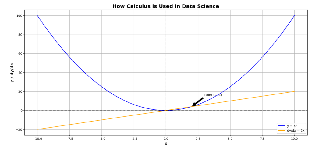
When people start exploring data science, they often think about coding, algorithms, and machine learning models. However, behind all these techniques lies mathematics, and particularly calculus plays a crucial role in shaping how we analyze data and build predictive models. Let’s break down how calculus for data science is used, especially focusing on derivatives, integrals, and multivariable calculus, which are foundational for optimization and predictive modeling.
Derivatives and Integrals in Data Science
We’ve touched on derivatives in a previous post, and they are important in understanding how a function changes. To recap, derivatives help us understand the rate of change—which is extremely valuable in data science when we want to optimize models.
Example:
When you’re creating a machine learning model, your goal is to reduce the cost function. This function measures how well your model fits the data.
To understand how to improve the model, you look at the derivative of the cost function. The derivative tells you how the error changes when you adjust the model’s parameters.
This is where gradient descent comes in. It’s an optimization technique that uses these derivatives to help you find the lowest possible error. By applying gradient descent, you can make small adjustments to the model until you reach a point where the error is minimized, leading to a better-performing model.
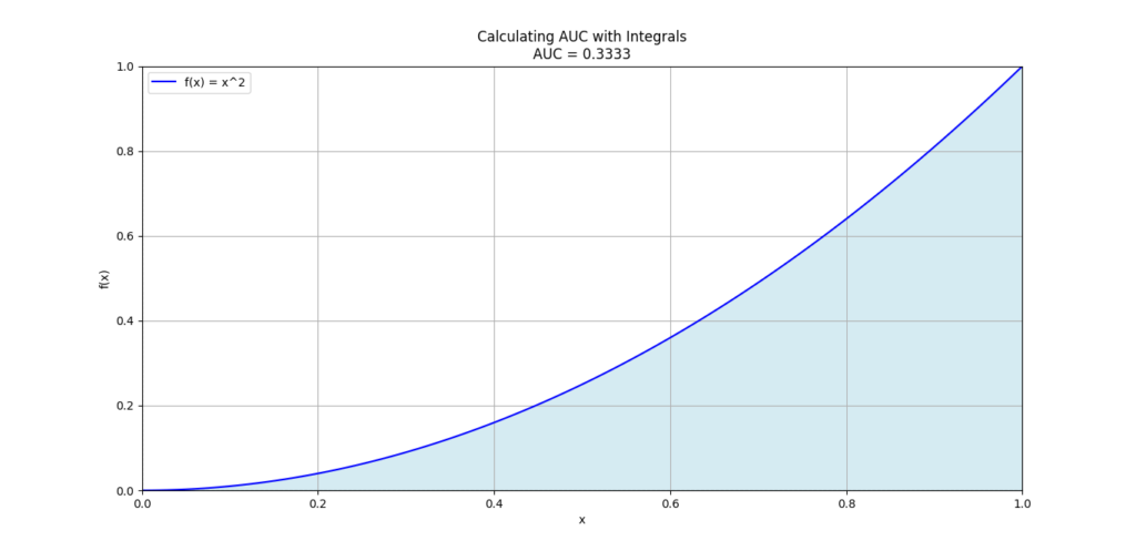
Integrals, on the other hand, allow us to calculate the area under curves. In data analysis, integrals come into play when we want to summarize data trends over time, or more commonly, when we measure the total effect of variables in a model.
Example:
In AUC (Area Under the Curve) calculations, which are crucial in classification models, integrals help quantify how well the model is performing by comparing true positives and false positives.
Why Advanced Calculus is Key for Model Optimization
The calculus for data science journey doesn’t stop at basic derivatives and integrals. To fine-tune complex models and make them more accurate, we need to apply advanced calculus concepts like multivariable calculus and gradient descent.
Gradient Descent and Calculus
Gradient descent lies at the core of many machine learning algorithms, serving as a powerful method to minimize the cost function. This is where calculus plays a crucial role:
- Gradient: This is a vector of partial derivatives that tells us how each parameter affects the model’s output.
- Descent: It helps us find the minimum value of the cost function by moving in the opposite direction of the gradient.
Using advanced calculus for optimization in data science, we can improve accuracy by refining the parameters of a model. For instance, if you’re training a deep learning model, each iteration uses calculus to adjust weights and biases so the model can learn better.
Example of Gradient Descent:
def gradient_descent(X, y, learning_rate, iterations):
    m = len(y)
    theta = np.zeros((X.shape[1], 1))
    for i in range(iterations):
        predictions = np.dot(X, theta)
        errors = predictions - y
        gradient = (1/m) * np.dot(X.T, errors)
        theta = theta - learning_rate * gradient
    return theta
This code demonstrates how gradient descent works: adjusting parameters (in this case, theta) based on the gradient of the error.
The Role of Multivariable Calculus
In real-world data, many models have several inputs. This is where multivariable calculus becomes useful for optimizing these models.
Unlike basic calculus, which focuses on a single variable, multivariable calculus allows us to work with multiple variables that affect each other.
To understand how each variable impacts the overall outcome, we use partial derivatives. These partial derivatives show us the effect of changing one variable while keeping the others constant. This way, we can see how each individual input influences the results, helping us make better decisions when building our models.
How Calculus Improves Predictive Modeling
Calculus plays an important role in predictive modeling. When we use models like linear regression or more complex neural networks, our goal is to predict outcomes based on input data.
Calculus for data science helps us fine-tune these models. It allows us to adjust weights and biases, which are the parameters that influence the predictions. By making these adjustments, we can improve the accuracy of our predictions and make our models more effective.
Calculating AUC with Integrals
In classification problems, especially in binary classification, the Area Under the Curve (AUC) is used to evaluate model performance. The AUC gives us a sense of how well the model distinguishes between the classes. Here, integrals come into play because AUC is essentially the integral of the ROC curve, which plots the true positive rate against the false positive rate.
Why You Should Care About Calculus for Data Science:
Here are some specific reasons why calculus for data science is critical:
- Model Accuracy: Calculus allows us to fine-tune parameters, making models more accurate and efficient.
- Optimization: Tools like gradient descent are impossible without a solid understanding of calculus.
- Predictive Power: Advanced calculus helps improve models that predict outcomes based on multiple variables.
- AUC and ROC Curves: Understanding integrals helps us measure a model’s performance using AUC in classification tasks.
Must Read
- PyTorch Debugging Checklist: A Systematic Framework to Fix Models That Won’t Learn
- Why sorted() Is Safer Than list.sort() in Production Python Systems
- Monotonic Sequence in Python: 7 Practical Methods With Edge Cases, Interview Tips, and Performance Analysis
- How to Check if Dictionary Values Are Sorted in Python
- Check If a Tuple Is Sorted in Python — 5 Methods Explained
Integrals in Data Science
When we talk about calculus for data science, many people focus on derivatives, but integrals are just as crucial. They allow us to handle continuous data and make sense of complex mathematical models, especially in probability and machine learning. Let’s explore how integrals contribute to various tasks like evaluating machine learning models, calculating probability densities, and improving classification algorithms.
The Role of Integrals in Machine Learning
When it comes to machine learning models, there’s a hidden mathematical powerhouse working behind the scenes—integrals. Though they may sound intimidating, integrals are just a way of adding up small parts to understand a whole. In machine learning, they’re especially useful when we deal with probabilities and model evaluation.
Let’s walk through the key mathematical ideas of integrals and how they impact machine learning in a more understandable way. If you’re exploring calculus for data science, this is your starting point.
What Are Integrals?
In simple terms, an integral helps us calculate the total amount or area under a curve. Imagine you’re trying to measure the area of a plot of land with uneven terrain. You could break it up into small pieces and add them up. That’s essentially the purpose of integrals with continuous data: they sum up all the small parts to determine a total.
For example, if you have a graph that represents the speed of a car over time, the integral of that graph would give you the total distance traveled. This idea is crucial in machine learning models, where we deal with probabilities and data distributions.
Integrals in Probability Density Functions (PDFs)
Understanding PDFs
A Probability Density Function (PDF) tells us how likely it is for a variable to have a certain value. The tricky part is that in continuous distributions, the chance of the variable being exactly one specific value is usually zero. Instead, we focus on the probability of the variable falling within a certain range of values, and that’s where integrals come in.
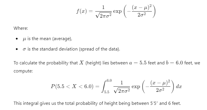
Let’s imagine that we are studying the height of people in a population. Heights follow a normal distribution (a bell-shaped curve), and we want to know the probability that someone is between 5’5” and 6 feet tall. Since height is a continuous variable, we can’t just list all possible values. Instead, we need to integrate the PDF over the range we care about.
Integrals for Calculating Probabilities
In continuous probability distributions, we cannot assign a specific probability to an exact point. Instead, we use integrals to calculate the probability that the variable lies between two points. This is done by integrating the PDF over that range.
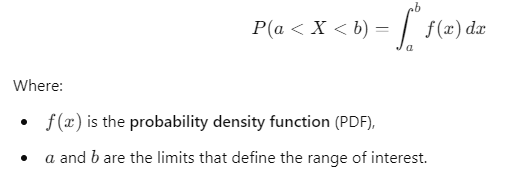
This integral calculates the total area under the curve between a and b, which gives us the probability that the variable X falls within that interval.
Example: Normal Distribution
Let’s use the normal distribution, a common continuous distribution used in many fields of statistics and probability:
Expected Value and Integrals
The expected value of a continuous random variable is another important concept in calculus for data science. The expected value tells us the long-term average or mean of a random variable. For continuous random variables, it’s calculated using an integral.
The expected value E[X] is given by:
![A formula representing the expected value E[X] of a random variable X, calculated by integrating the product of X and its probability density function (PDF) over all possible values.](https://emitechlogic.com/wp-content/uploads/2024/10/expected-value.png)
This equation integrates the product of the random variable x and its PDF over the entire range of possible values.
Example: Expected Value of a Normal Distribution
Let’s say we have a normal distribution for heights with a mean μ=5.8 feet and a standard deviation σ=0.3. The expected value would simply be the mean in this case, but the formula shows how the expected value is the weighted average of all possible values of x, weighted by their likelihood.
Cumulative Distribution Function (CDF)
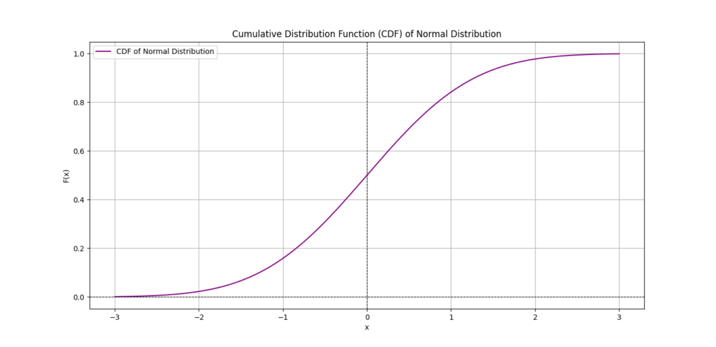
In addition to PDFs, Cumulative Distribution Functions (CDFs) are another area where integrals are essential. A CDF gives the probability that a random variable X is less than or equal to a particular value x. The formula for a CDF is:

This integral sums up all the probabilities from −∞ to x, giving the cumulative probability up to that point. CDFs are useful when we need to know the total probability of an event occurring below a certain threshold.

Why Are CDFs Important?
In machine learning models, CDFs are used in algorithms like logistic regression to calculate the probability of a certain class (like “positive” or “negative”). They also come in handy for ranking problems where you need to measure how well your model separates different outcomes.
Integrals in Statistics for Estimating Parameters
Integrals also play a role in estimating parameters like means and variances for continuous data. For example, to estimate the variance σ2, we use integrals:
![A formula for calculating the variance using the expected value of X² (E[X²]) and the square of the expected value of X, with integrals for continuous data.](https://emitechlogic.com/wp-content/uploads/2024/10/Integrals-in-Statistics.png)
By integrating the squared values of x multiplied by their probability, we get the expected value of X2. Subtracting the square of the mean gives us the variance, which measures how spread out the values of X are.
Integrals in Machine Learning Model Evaluation
Loss Functions and Model Optimization
When building machine learning models, you’ll often hear about loss functions. A loss function measures how far off a model’s predictions are from the actual values. One common example is Mean Squared Error (MSE), which looks like this for discrete data:

In this form, the MSE becomes a continuous sum (an integral) of the squared errors over all possible values of x. Minimizing this error helps us train our model to make better predictions.
Integrals in Support Vector Machines (SVMs)
For SVMs, integrals are used to find the best boundary (or hyperplane) that separates different classes in the data. This involves optimizing a function that depends on the data points in the feature space. Once again, integrals help sum up these continuous optimizations.
Simple Python Example
Let’s see a simple Python example using the SciPy library to compute an integral for a normal distribution’s CDF.
from scipy.integrate import quad
import numpy as np
import math

# Define the PDF for a normal distribution
def normal_pdf(x, mu, sigma):
    return (1 / (sigma * np.sqrt(2 * np.pi))) * np.exp(-0.5 * ((x - mu) / sigma)**2)

# Calculate the CDF for a given value (e.g., probability that X <= 6.0)
mu = 5.8  # Mean height
sigma = 0.3  # Standard deviation
cdf_result, _ = quad(normal_pdf, -np.inf, 6.0, args=(mu, sigma))

print("The probability that height is <= 6 feet is:", cdf_result)
This code computes the CDF for a normal distribution with a mean of 5.8 and a standard deviation of 0.3. It calculates the probability that a height is less than or equal to 6 feet by integrating the PDF.
Using Integrals to Improve Classification Algorithms
In data science, classification models are a powerful tool, especially when dealing with tasks like spam detection, image classification, or disease diagnosis. To understand how well a model performs, we use various metrics, such as the ROC curve and AUC (Area Under the Curve). What’s fascinating is that integrals help us calculate these metrics, offering insights into a model’s accuracy.
Let’s explore how integrals are applied in classification algorithms to calculate these important evaluation metrics.
What is an ROC Curve?
The ROC curve (Receiver Operating Characteristic) is a graph that shows the performance of a classification model at different threshold settings. It plots two main parameters:
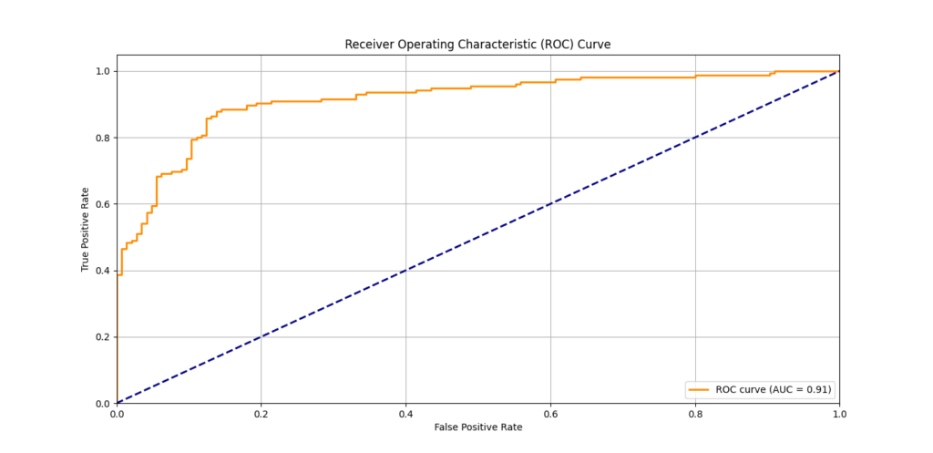
This ROC curve evaluates the performance of a binary classification model by plotting the True Positive Rate (sensitivity) against the False Positive Rate. The orange curve represents the ROC, and the diagonal dashed line indicates random guessing. The Area Under the Curve (AUC) score is 0.85, indicating a good performance of the model.
- True Positive Rate (TPR): How many positive instances are correctly classified.
- False Positive Rate (FPR): How many negative instances are incorrectly classified as positive.
These are plotted on the y-axis and x-axis, respectively. The curve gives us a sense of how well the model distinguishes between classes, with a higher curve indicating better performance.
But how do integrals fit in?
Calculating the AUC with Integrals
AUC stands for Area Under the Curve, and it’s one of the most important metrics used to evaluate classification models. A perfect classifier would have an AUC of 1.0, meaning it perfectly distinguishes between the two classes.
Now, the AUC represents the area under the ROC curve, and calculating this area is exactly where integrals come into play. To get the AUC, we compute the area under the ROC curve from 0 to 1 along the False Positive Rate (FPR) axis.
The AUC is formally calculated using the following integral:

This formula tells us to integrate the True Positive Rate (TPR) with respect to the False Positive Rate (FPR). In simpler terms, we’re summing the areas beneath the curve to get a single number that reflects the overall performance of the classifier.
Example: ROC Curve and AUC Calculation
Let’s imagine we’re using a classifier to detect whether an email is spam or not. The ROC curve generated from this classifier looks like a smooth curve, and we want to calculate the AUC. Using integrals, we calculate the area under the ROC curve, which may look something like this:

In practice, you would use numerical integration methods, often done with Python or other tools, to compute this area. Here’s a Python example using SciPy to compute the AUC:
from sklearn import metrics
import numpy as np

# Example data for FPR and TPR
fpr = np.array([0.0, 0.1, 0.4, 0.6, 1.0])
tpr = np.array([0.0, 0.6, 0.8, 0.9, 1.0])

# Calculate AUC using trapezoidal rule
auc = metrics.auc(fpr, tpr)
print(f"The AUC of the classifier is: {auc}")
This script calculates the AUC using the trapezoidal rule, which is a numerical method for estimating the area under a curve—just another way integrals come into play.
Precision-Recall Curve: Another Application of Integrals
Besides the ROC curve, the Precision-Recall Curve is another useful tool for evaluating classification models, especially when dealing with imbalanced datasets.
The Precision-Recall Curve plots precision (the ratio of true positives to all predicted positives) against recall (the ratio of true positives to actual positives). The area under this curve (AUC for Precision-Recall) can also be calculated using integrals.
In this case, the area under the Precision-Recall curve is computed by:

Where:
- P(R) is the precision as a function of recall,
- dR represents changes in recall.
Improving Model Performance Using AUC
Integrals in classification algorithms help data scientists assess their models and make improvements. For example:
- Threshold selection: By examining the ROC curve, we can pick the best threshold that balances false positives and true positives.
- Model comparison: If you want to compare two models, the AUC gives you a simple way to see which one performs better overall.
- Handling imbalanced datasets: In cases where one class dominates, the Precision-Recall curve and its integral-based AUC give more meaningful insights than accuracy alone.
Real-World Example: Medical Diagnostics
In the healthcare field, classification models are often used to predict diseases. Take, for example, a model predicting whether a patient has cancer based on diagnostic features.
- The ROC curve will help you see how well the model distinguishes between healthy and sick patients.
- The AUC value tells you the overall effectiveness of the model. If the AUC is close to 1, the model is highly reliable.
By integrating these concepts, data scientists can provide more accurate predictions and make better clinical decisions.
Multivariable Calculus for Data Science
What is Multivariable Calculus?
When we think about calculus, many people know about the kind that works with one variable. For example, we might calculate how fast a simple function like f(x) = x^2 changes. However, the real world is usually more complicated and involves many variables that affect each other. This is where multivariable calculus is useful. It builds on single-variable calculus and helps us work with functions that depend on multiple variables.
In data science, where we often deal with datasets with numerous features or dimensions, understanding multivariable calculus becomes crucial. It helps with tasks such as optimizing machine learning models, calculating gradients, and understanding complex functions in multiple dimensions. So, let’s break it down.
Expanding to Multiple Variables
In single-variable calculus, a function depends on just one variable. For example:
f(x)=x^2
Here, x is the input, and we can calculate derivatives and integrals based on that single input. But what if we have a function that depends on more than one variable? For instance:
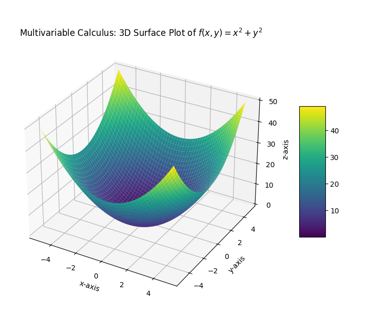
f(x, y) = x^2 + y^2
Now, we’re dealing with a function of two variables, x and y. This expansion is the core idea behind multivariable calculus. It allows us to:
- Analyze how a change in one variable affects the outcome while keeping other variables constant.
- Understand how multiple variables together influence a result, such as the behavior of a dataset with numerous features in machine learning.
In data science, many algorithms work with functions that have several variables, making multivariable calculus essential for optimization and understanding how models behave.
Partial Derivatives: A Key Concept
In multivariable calculus, the concept of partial derivatives becomes important. A partial derivative measures how the function changes as one variable changes, while keeping the other variables constant.
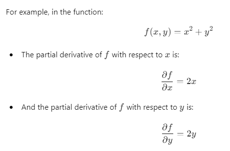
This means that we can study the rate of change in f(x,y) as x or y changes individually. These partial derivatives are crucial for understanding and optimizing machine learning models, where each feature in the data may represent a different dimension.
Gradient: The Direction of Steepest Ascent
One of the key tools in multivariable calculus is the gradient. The gradient is a vector that shows the direction in which a function increases the fastest. It’s created by taking the partial derivative of the function for each variable.

In data science, the gradient helps us optimize models. For instance, in gradient descent—an algorithm used to minimize the loss function in machine learning—the gradient tells us the direction to move to reduce error.
Multivariable Calculus in Data Science
Here’s how multivariable calculus plays a key role in data science:
- Gradient Descent: This is an optimization algorithm used in training machine learning models. The algorithm uses the gradient to iteratively adjust the model parameters to minimize the error.
- The loss function in machine learning often depends on multiple variables (parameters), and multivariable calculus helps us compute the gradient and move in the direction that reduces the loss.
- Cost Functions: These functions, which measure the error between the model’s prediction and the actual values, depend on multiple parameters. Multivariable calculus helps us understand how changing one parameter affects the overall cost.
- Backpropagation in Neural Networks: This process involves calculating the gradient of the error with respect to each weight in the network. This is a direct application of multivariable calculus since the network’s error depends on many variables (weights).
- Optimization: Many machine learning tasks involve optimizing functions that depend on multiple variables. Whether we’re tuning hyperparameters or minimizing loss functions, multivariable calculus is what makes these optimizations possible.
Example: Gradient Descent in Machine Learning
To show how multivariable calculus helps in data science, let’s look at a simple example: gradient descent.
Imagine we have a cost function for a model that depends on two parameters, θ1 and θ2:
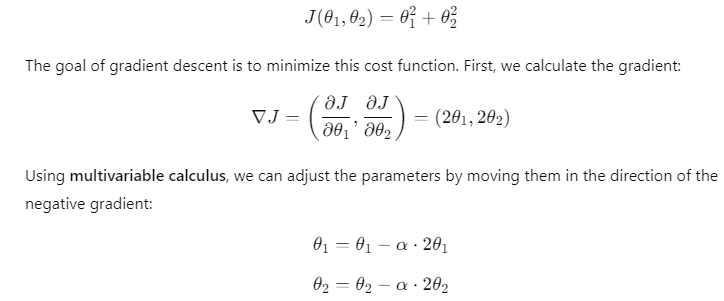
Where α is the learning rate. This iterative process, powered by multivariable calculus, helps the model gradually reduce error and improve performance.
Real-Life Applications
In real-world applications, multivariable calculus is used across various fields, from data science to physics and economics. For instance:
- In machine learning: Multivariable calculus is the backbone of algorithms like linear regression, logistic regression, and neural networks.
- In optimization problems: It helps us solve complex problems where multiple variables influence the outcome.
Differential Equations in Data Science
In data science, understanding the role of differential equations can be a game-changer. They are mathematical tools used to describe how things change. Whether you’re modeling population growth, studying how a system evolves over time, or improving machine learning algorithms, differential equations can help. For those learning calculus for data science, this topic offers valuable insights into how changes over time or across variables are captured mathematically.
What Are Differential Equations?
Differential equations are used to describe how one quantity changes in relation to another. They often include derivatives, which represent rates of change for one or more variables. A common example is the equation for exponential growth:

Differential equations can be categorized into:
- Ordinary differential equations (ODEs): Involve functions of one variable.
- Partial differential equations (PDEs): Involve functions of multiple variables.
Why Are Differential Equations Important in Data Science?
Data science deals with systems that evolve over time or interact with multiple variables. Differential equations help us model these dynamics. Here are a few areas where differential equations shine:
- Predictive modeling: Differential equations help model how a system evolves, like predicting disease spread or stock market trends.
- Machine learning: Algorithms such as gradient descent, used in training machine learning models, rely on differential equations to update parameters and minimize errors.
- Natural language processing: In dynamic models of language or in text generation tasks, differential equations help track changes in word usage over time.
- Physics-based modeling: Many real-world systems (e.g., climate modeling, financial forecasting) use differential equations to predict future states based on current observations.
Solving Differential Equations in Data Science
In data science, we often use numerical methods to solve differential equations. Since many real-world problems are too complex to solve analytically, computational tools step in to help. Below are some common methods for solving ordinary differential equations (ODEs):
- Euler’s Method: A simple, step-by-step approach to approximate solutions.
- Runge-Kutta Methods: These are more accurate than Euler’s method and widely used in practice.
- Finite Difference Methods: Often used for solving partial differential equations (PDEs), especially when dealing with multiple variables.

To solve this, we separate the variables and integrate:
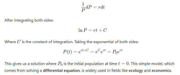
Differential Equations in Machine Learning
Differential equations play a crucial role in training machine learning models. In particular, they are the mathematical backbone of optimization techniques used to minimize the error between a model’s prediction and actual results.
Gradient Descent as a Differential Equation
In machine learning, the gradient descent algorithm uses derivatives (a type of differential equation) to minimize a cost function. The idea is to update the model’s parameters step by step in the opposite direction of the gradient. This process is mathematically described as:

Partial Differential Equations (PDEs) in Data Science
While ordinary differential equations (ODEs) involve one variable, partial differential equations (PDEs) deal with multiple variables. PDEs are common in physics-based data science applications, such as climate models or financial systems.
An example of a PDE is the heat equation, which models the distribution of heat (or energy) over time:
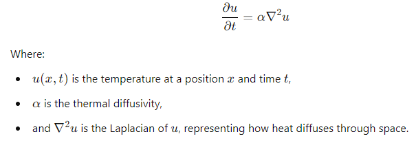
PDEs like this are solved using numerical methods such as finite difference or finite element methods. They are essential when dealing with large-scale systems that evolve over time, which is common in fields like weather prediction and financial modeling.
Real-World Applications of Differential Equations in Data Science
Here are some key applications where differential equations are used in data science:
- Predictive analytics: Differential equations help model systems that change over time, such as forecasting stock prices or predicting disease outbreaks.
- Neural networks: In training deep learning models, differential equations guide the backpropagation process to optimize model weights.
- Control systems: PDEs and ODEs are often used in autonomous systems (e.g., self-driving cars) to model and control behavior.
- Physics simulations: Systems like weather models, climate predictions, and even sports simulations rely on differential equations to simulate reality accurately.
Vector Calculus and Its Relevance in Data Science
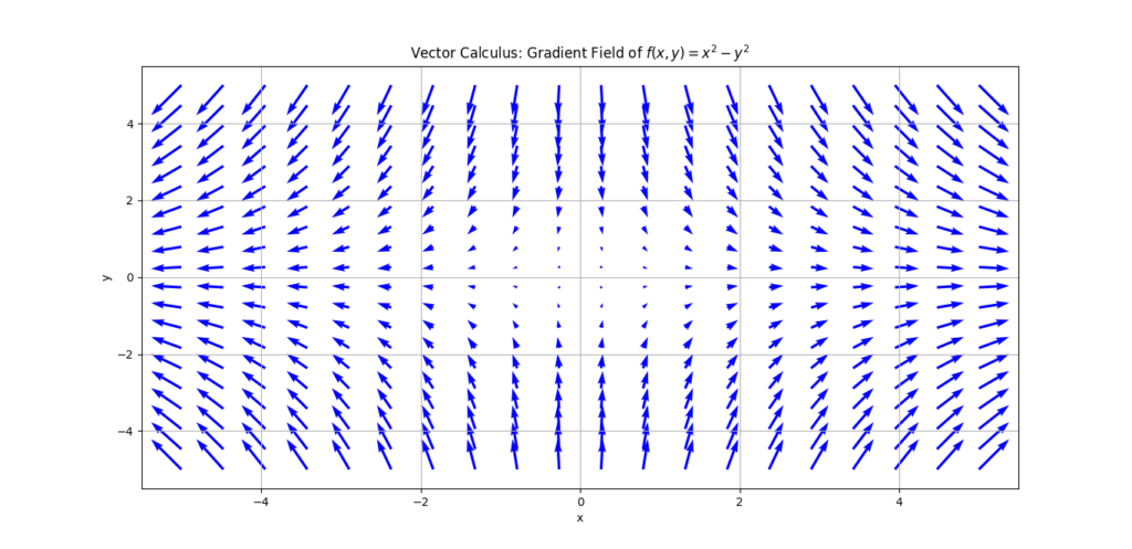
Vector calculus is a crucial mathematical tool, especially for those working in data analysis and machine learning. It extends the ideas of single-variable calculus to functions of multiple variables, where both input and output are vectors. For anyone diving into neural networks or deep learning, vector calculus for data analysis becomes an essential area of study, as it helps in understanding how optimization and backpropagation work.
Introduction to Vector Calculus
Vector calculus is a branch of math that focuses on vector fields, which involve both direction and magnitude. Instead of just working with numbers (as in regular calculus), vector calculus deals with functions that take in and return vectors—quantities that have both size and direction. It involves operations like differentiation and integration, but applied to these more complex vector functions rather than simple numerical ones.
Why does this matter in data science? In many data analysis applications, variables can depend on multiple factors. Vector calculus helps in analyzing how these variables interact and change. In the context of neural networks and deep learning, vector calculus supports operations like finding gradients, which are fundamental for optimizing models.
Key Concepts in Vector Calculus:
- Gradient: Describes how much and in what direction a function is increasing or decreasing.
- Divergence: Measures the “outflow” of a vector field.
- Curl: Represents the rotation or “twisting” of a vector field.
Vector Calculus in Neural Networks
The gradient is a fundamental concept in neural networks. It represents the direction and rate of change of a function with respect to its inputs. In deep learning, the gradient helps optimize weights and biases to reduce error during training.
Gradients and Backpropagation
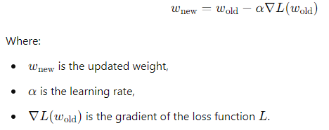
In neural networks, backpropagation is the process of updating model parameters by calculating the error’s gradient concerning each weight. This involves computing the partial derivatives of the error function. Here’s where vector calculus steps in:
- Gradient descent: This optimization algorithm uses the gradient to adjust the weights step-by-step. Mathematically, the weight update rule looks like:
Jacobian matrices: These matrices capture the gradients for multiple outputs and multiple inputs, which is particularly useful in multilayer neural networks where the relationships between inputs and outputs become complex.
Example: Backpropagation Using Gradients
Let’s say we have a simple neural network. During training, the error between the predicted output and the actual output is calculated. Using the gradient, the network adjusts its weights to minimize this error.
If the loss function L(w) depends on the weight w, the network computes the gradient ∇L(w), which tells us in which direction to update the weight to minimize the loss.
In short, vector calculus in neural networks forms the mathematical foundation for backpropagation, helping us improve model accuracy.
Divergence, Curl, and Their Role in Data Science
Another critical area of vector calculus for data analysis is understanding the behavior of vector fields through divergence and curl. Both concepts provide ways to measure how vector fields behave and change.
What is Divergence?
Divergence measures the magnitude of a field’s source or sink at a given point. It tells us whether vectors are “flowing out” or “converging inward” in a space.
For instance, in data science applications like modeling fluid dynamics or traffic flow, divergence can help predict whether a system is expanding or compressing in a region. In simple terms, divergence indicates whether the vector field is dispersing (positive divergence) or converging (negative divergence).
What is Curl?
Curl represents the rotation or twisting of a vector field. It measures how much a vector field is “circulating” around a point, rather than flowing in a straight line. This is useful in analyzing systems with rotational movement, like weather patterns or electric fields.
In data science, we can use curl to model and understand flow patterns in various scenarios, such as how information or influence propagates across social networks or how resources like water or electricity flow through a network.
Real-World Applications:
- Divergence in Data Science: Helps model traffic patterns, population dynamics, or heat diffusion.
- Curl in Data Science: Models phenomena like wind patterns in weather simulations or rotation in fluid systems.
Example: Using Vector Calculus in a Neural Network
Let’s go back to neural networks and how vector calculus operates behind the scenes. Consider a neural network with a loss function L, which we want to minimize by adjusting the weight matrix W.
- First, we compute the gradient of the loss function, ∇L(W).
- Next, we use gradient descent to update the weights:

The Jacobian provides a more detailed view of how multiple variables interact, which is especially useful in complex deep learning systems.
Numerical Methods for Calculus in Data Science
![A plot illustrating the Trapezoidal Rule for numerical integration of the function 𝑓 ( 𝑥 ) = sin ( 𝑥 ) f(x)=sin(x) over the interval [ 0 , 𝜋 ] [0,π]. The red curve represents the sine function, while blue trapezoids filled with a transparent color approximate the area under the curve.](https://emitechlogic.com/wp-content/uploads/2024/10/Trapezoidal-Rule-1-1024x497.png)
Numerical methods offer powerful techniques for solving complex mathematical problems, especially when analytical solutions are unavailable. In the context of data science, these methods are used to approximate integrals and derivatives—both fundamental operations in calculus—helping to optimize machine learning models and understand large datasets. Through this guide, we’ll explore some widely used numerical methods for calculus in data science and see how they support tasks such as gradient calculation and model optimization.
Introduction to Numerical Integration and Differentiation
In many real-world problems, it is difficult to compute integrals or derivatives directly using traditional calculus methods. This is where numerical methods come into play. They allow us to approximate these values with great precision. Two popular techniques for solving integrals numerically are the Trapezoidal Rule and Simpson’s Rule.
Trapezoidal Rule
The Trapezoidal Rule is a method used to approximate the area under a curve by dividing it into trapezoids instead of the exact shape of the curve. It works especially well when the function isn’t too curvy.
Formula:
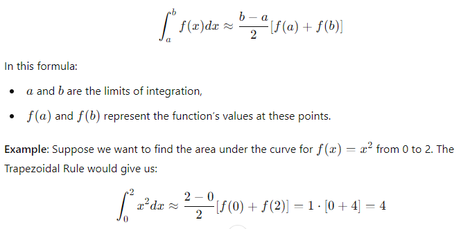
Though this is an approximation, it is often close enough for practical applications.
Simpson’s Rule
Simpson’s Rule is another method for numerical integration, but it tends to be more accurate because it uses parabolas to approximate the curve. It is especially useful for functions that curve more dramatically.
Formula:

Compared to the Trapezoidal Rule, Simpson’s Rule provides a better approximation in this case.
Applications of Numerical Methods in Machine Learning
In machine learning, numerical methods play an essential role, particularly in optimization tasks. Models often rely on gradient-based algorithms like gradient descent to minimize error functions. These gradients are not always easy to compute analytically, which is where numerical approximations become invaluable.
Numerical Methods in Gradient Descent
Gradient descent is the cornerstone of many machine learning algorithms. This optimization algorithm helps models update their parameters (like weights) by following the steepest descent in error. When computing the exact gradient becomes infeasible, numerical differentiation can help.
For example, in some neural networks, calculating derivatives with respect to every parameter might require approximations. One commonly used method is finite differences, where the gradient is estimated by evaluating small changes in the function:

Where h is a small value. This allows us to approximate the slope of the function without requiring complex symbolic differentiation.
Complex Integrals in Machine Learning
Sometimes, integrals arise in machine learning models, especially in probabilistic models such as Bayesian networks. Many of these integrals do not have analytical solutions and must be approximated using numerical methods. For example, Monte Carlo integration is frequently used to approximate high-dimensional integrals by taking random samples from the distribution:

Where N is the number of samples, and xi are the random points sampled. This approach is useful in high-dimensional problems, such as optimizing deep learning models.
The Latest Advancements in Calculus for Data Science
In the rapidly growing field of data science, the role of calculus cannot be overstated. From optimizing machine learning models to refining reinforcement learning strategies, calculus is fundamental. Recent advancements in automatic differentiation, symbolic computation tools, and the application of calculus in reinforcement learning have made it easier for data scientists to work with complex models, leading to more accurate results and better optimization.
Automatic Differentiation in Machine Learning
One of the significant advancements in deep learning has been the rise of automatic differentiation tools like TensorFlow and PyTorch. These frameworks handle the complex task of calculating derivatives in multi-layered models with minimal manual intervention. Traditionally, calculating derivatives for large models involved tedious manual work, particularly when dealing with nested functions and complex layers.
Automatic differentiation simplifies this by systematically applying the chain rule to compute derivatives, which are essential for gradient descent—a common optimization method used to minimize the loss function in neural networks.
Example of Automatic Differentiation in PyTorch
Let’s take a simple example of how automatic differentiation works in PyTorch:
import torch

# Create a tensor
x = torch.tensor(2.0, requires_grad=True)

# Define a function
y = x**3 + 5*x

# Compute the derivative
y.backward()

# Print the gradient
print(x.grad)  # Output: tensor(17.)

Key points about automatic differentiation:
- It efficiently handles complex models, such as those found in deep learning.
- It calculates gradients automatically, which are used to update model parameters during training.
- Tools like TensorFlow and PyTorch have revolutionized model optimization by incorporating this feature.
Automatic differentiation in deep learning makes it possible to focus on model architecture and performance without getting bogged down by the complexities of derivative calculation, which is particularly useful in Calculus for Data Science.
Symbolic Computation Tools in Data Science
Another exciting development in data science is the use of symbolic computation tools for handling more abstract and algebraic calculus operations. Tools like SymPy (in Python) and Mathematica can perform symbolic differentiation, integration, and even equation solving, providing a way to manipulate equations algebraically rather than numerically.
Symbolic computation tools for calculus in data science are highly useful in both theoretical research and practical applications. By solving symbolic expressions, data scientists can gain deeper insights into model behavior and optimize complex systems more effectively.
Example of Symbolic Differentiation with SymPy
import sympy as sp

# Define a symbolic variable
x = sp.Symbol('x')

# Define a function
f = x**3 + 5*x

# Perform symbolic differentiation
dfdx = sp.diff(f, x)

# Output the derivative
print(dfdx)  # Output: 3*x**2 + 5
In this example, SymPy provides the exact symbolic derivative of the function f(x)=x3+5x. This can be especially valuable when working with optimization problems in machine learning or any domain where analytical insights are needed.
Benefits of symbolic computation tools:
- They enable exact solutions to calculus problems, offering deeper theoretical insights.
- They are highly beneficial in research, where symbolic solutions can help uncover new trends or patterns.
- These tools can handle a range of mathematical operations, from differentiation to integration and solving differential equations.
In the realm of Calculus for Data Science, symbolic computation plays a crucial role in the optimization and analysis of algorithms.
Calculus in Reinforcement Learning and AI
Reinforcement learning (RL) is a subset of artificial intelligence (AI) that focuses on training agents to make decisions by maximizing some notion of cumulative reward. Calculus plays a central role in reinforcement learning by helping to optimize the reward function and by computing gradients that guide policy updates.
One of the primary uses of calculus in reinforcement learning and AI is in the calculation of gradients that dictate how an agent’s actions impact future rewards. By leveraging calculus, specifically through methods like policy gradients, reinforcement learning algorithms can effectively improve decision-making over time.
Gradient Calculation in Reinforcement Learning
In many RL algorithms, we optimize the agent’s behavior by using stochastic gradient descent. This method adjusts the parameters of the agent’s policy to maximize expected reward, relying heavily on gradients calculated via automatic differentiation or symbolic methods.
For example, policy gradient methods use calculus to compute how small changes in a policy will affect the cumulative rewards.
Divergence and Curl in Data Science
In certain data science applications, especially those involving flow models or vector fields, concepts like divergence and curl become very important.
- Divergence measures the magnitude of a source or sink at a given point in a vector field. In simpler terms, it tells us how much a vector field spreads out or converges at a point.
- Curl describes the rotation of a vector field around a point. It shows whether there is any swirling motion at that point.
These concepts are particularly useful in physics-based models, fluid dynamics simulations, or fields like computational biology, where data scientists model systems with directional flow.
Practical Examples of Using Advanced Calculus in Data Science
The use of calculus in data science opens doors to solving intricate problems like optimization and integration, which play a crucial role in machine learning and predictive modeling. Here, we’ll dive into practical applications of advanced calculus with real examples from data science.
Python Code Example for Solving Integrals in Data Science
Numerical integration plays a vital role in data science, especially when dealing with probability distributions, loss functions, or optimization. Often, we encounter integrals that cannot be solved analytically, requiring us to resort to numerical methods.
For example, in data science, we may need to integrate a function to find the area under a curve representing some distribution. Python libraries such as SciPy and SymPy make it easy to perform this kind of calculus.
Solving Integrals Using SciPy
Let’s say we need to calculate the integral of f(x) = x^2 between x=0 and x=1, which is a common task in estimating continuous data:
import scipy.integrate as integrate

# Define the function
def f(x):
    return x**2

# Perform the integration
result, error = integrate.quad(f, 0, 1)

print(f"Result: {result}, Error: {error}")
In this example:
quadfrom the SciPy library computes the definite integral of the function f(x) = x^2 between 0 and 1.- The output provides both the integral’s result and an estimation of the error, which is particularly useful when dealing with numerical integration.
Python code for solving integrals in data science allows you to approach complex problems where analytical solutions are impossible or difficult.
Case Study: Multivariable Optimization for Model Training
In machine learning, multivariable optimization is essential for improving model performance. We often deal with complex objective functions that depend on multiple parameters—ranging from weights in a neural network to the coefficients in linear regression.
Let’s walk through a case study that illustrates how multivariable calculus can be applied in model training or hyperparameter tuning.
Problem: Tuning Hyperparameters of a Regression Model
Consider a machine learning model tasked with predicting house prices. The goal is to optimize multiple parameters, such as learning rate, regularization term (λ), and the number of iterations.
We want to minimize the cost function—the function that measures the error between predicted and actual values—using gradient descent, an algorithm driven by calculus. The cost function for ridge regression is:
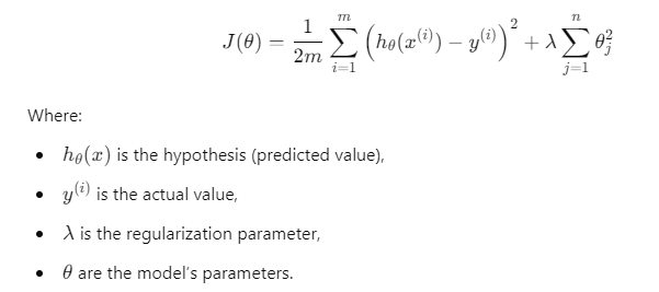
This cost function depends on several parameters, making multivariable optimization essential.
Steps for Multivariable Optimization
- Define the objective: We need to find the parameters that minimize the cost function.
- Compute gradients: The gradients of the cost function with respect to each parameter are calculated. In ridge regression, this would involve the partial derivatives of J(θ) with respect to each θ.
- Update parameters: Using gradient descent, we iteratively adjust the parameters based on the computed gradients, following the direction that minimizes the cost.
Python Code for Multivariable Optimization
Here’s how you might implement gradient descent to optimize a simple linear regression model with multiple features:
import numpy as np

# Define the cost function for linear regression
def cost_function(theta, X, y):
    m = len(y)
    return (1 / (2 * m)) * np.sum((X.dot(theta) - y) ** 2)

# Gradient descent function
def gradient_descent(X, y, theta, learning_rate, iterations):
    m = len(y)
    cost_history = np.zeros(iterations)

    for i in range(iterations):
        theta = theta - (1/m) * learning_rate * X.T.dot(X.dot(theta) - y)
        cost_history[i] = cost_function(theta, X, y)

    return theta, cost_history

# Initialize parameters
X = np.array([[1, 1], [1, 2], [1, 3]])  # Features
y = np.array([1, 2, 3])  # Target values
theta = np.zeros(2)  # Initial parameters
learning_rate = 0.01
iterations = 1000

# Run gradient descent
theta, cost_history = gradient_descent(X, y, theta, learning_rate, iterations)

print(f"Optimized Parameters: {theta}")
In this example:
- Gradient descent is applied to optimize the parameters θ0\theta_0θ0 and θ1\theta_1θ1 of a simple linear regression model.
- The cost function decreases with each iteration, improving the model’s performance.
Multivariable Optimization Key Insights:
- Multivariable optimization in data science is essential for tuning machine learning models and training algorithms.
- Gradient-based methods like gradient descent rely on calculus to find optimal parameter values.
- Multivariable optimization can be applied to tasks such as hyperparameter tuning, ensuring the model generalizes well to unseen data.
Conclusion: Why Mastering Advanced Calculus is Essential for Data Science Success
Advanced calculus plays a crucial role in data science. It forms the backbone of many key processes in machine learning and artificial intelligence. Whether you’re calculating derivatives for optimization or solving integrals in probabilistic models, calculus is vital for building efficient and accurate models.
Understanding advanced calculus helps data scientists dive deeper into how neural networks learn. It is essential for refining models using gradient-based methods and improving performance through multivariable optimization.
Tools like automatic differentiation and symbolic computation make calculus applications easier. However, a solid grasp of calculus concepts is needed to use these tools effectively.
In reinforcement learning, calculus is used to optimize reward functions. It is also key for solving integrals when working with continuous data distributions. To build scalable, high-performing solutions in data science and AI, advanced calculus is not just helpful—it’s essential.
Mastering calculus for data science will give you the skills to build models that tackle both current challenges and future innovations.
External Resources
MIT OpenCourseWare: Multivariable Calculus
- MIT’s free course on multivariable calculus dives into concepts like gradients, integrals, and partial derivatives, which are key to understanding calculus applications in data science.
- MIT OpenCourseWare – Multivariable Calculus
Stanford University: CS229 – Machine Learning
- This Stanford course includes discussions on calculus and its role in machine learning, particularly in optimization and training models.
- Stanford University – CS229: Machine Learning
SciPy Documentation: Numerical Methods
- The SciPy library is a Python tool widely used in data science. The documentation includes examples of numerical methods like integration and differentiation that are essential in machine learning.
- SciPy – Numerical Methods
FAQs
Why is advanced calculus important in data science?
Advanced calculus helps in optimizing machine learning models, calculating gradients for training algorithms like gradient descent, and handling multivariable functions in neural networks.
What calculus concepts are most used in data science?
Key concepts include derivatives (for optimization), integrals (for continuous data), partial derivatives (for multivariable functions), and gradients (for finding the direction of steepest ascent in functions).
How is multivariable calculus applied in machine learning?
Multivariable calculus is used to calculate partial derivatives and gradients, essential in training models with multiple features, adjusting weights, and minimizing error functions.
What tools can I use to apply calculus in data science?
Tools like TensorFlow, PyTorch (for automatic differentiation), SciPy (for numerical integration), and SymPy (for symbolic computation) are commonly used to apply calculus in data science.






Leave a Reply