Derivatives in Data Science: A Simple Guide to Calculus
Introduction to Derivatives in Data Science
Ever wondered how data scientists optimize models, predict trends, and make informed decisions? The secret lies in calculus, specifically derivatives. But don’t worry, you don’t need to be a math whiz to grasp it! In this guide, we’ll break down Derivatives in Data Science and show you how they’re used in data science. You’ll learn:
- How derivatives improve model accuracy
- Why optimization techniques rely on derivatives
- Real-world examples of derivatives in action
No prior calculus knowledge required! We’ll use simple language, relatable analogies, and practical examples to make derivatives accessible.
What to expect:
- Easy-to-understand explanations
- Visual illustrations and examples
- Code snippets in Python
Join us as we explore the fascinating world of calculus in data science. Discover how derivatives can enhance your data analysis skills and take your insights to the next level.
Introduction to Calculus in Data Science
What is Calculus?
Calculus is a branch of math. It focuses on how things change and accumulate. It has two main parts: derivatives and integrals.
Derivatives
- Definition: Derivatives show how fast something changes. For example, the speed of a car at a moment is a derivative. It tells us how position changes over time.
- Real-World Example: Think about a delivery service. It tracks how fast its vehicles go. By using derivatives, the company can see how quickly each vehicle moves. This helps them plan better routes.
Integrals
- Definition: Integrals measure the accumulation of quantities over an interval. They are often used to calculate areas under curves or the total accumulated value.
- Real-World Example: Picture a grocery store tracking the total sales over a month. Using integrals, the store can find out how much revenue was generated over that period by calculating the area under the sales curve.
Significance in Data Science
Calculus is important for building models and solving problems in data science. It helps data scientists predict outcomes and analyze trends.
- Mathematical Modeling: Data scientists use calculus to create models that describe complex systems. For example, a stock price prediction model uses derivatives to see how sensitive the price is to market changes.
- Problem-Solving: Calculus helps data scientists solve real-world problems. They can find key points in their models, which show optimal solutions or significant changes.
Why is Calculus Important for Data Science?
Data scientists should learn calculus for many reasons. Here are some key benefits:
- Optimization: Calculus helps with optimization techniques like gradient descent. This method reduces errors in models by adjusting parameters using derivatives.
- Predictive Modeling: Calculus aids in creating models that predict outcomes. For example, a marketing model may forecast customer behavior by analyzing how price changes affect sales.
- Gradient Descent: This algorithm uses derivatives to update model parameters step by step. By calculating the gradient (a vector of derivatives), data scientists find the fastest way to minimize errors.
Real-World Applications in Machine Learning and AI
Calculus is used in many machine learning algorithms and AI systems:
- Linear Regression: Data scientists use derivatives to minimize the cost function. This helps them find the best-fitting line through data points.
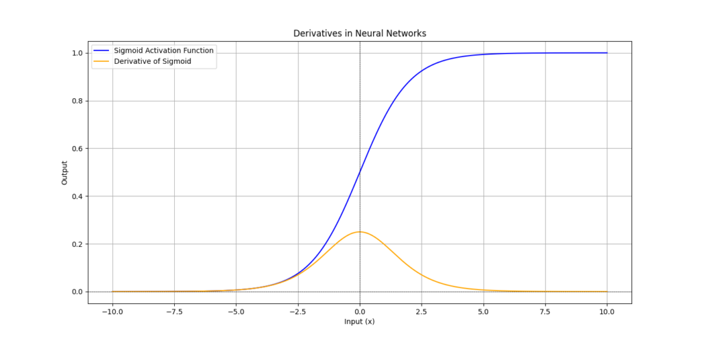
- Neural Networks: During training, derivatives calculate gradients for backpropagation. This process adjusts weights to improve predictions.
- Support Vector Machines (SVM): Calculus helps maximize the gap between classes by finding optimal hyperplanes.
Summary Table
| Concept | Definition | Real-World Application |
|---|---|---|
| Derivatives | Rate of change of a quantity | Speed of vehicles in delivery services |
| Integrals | Accumulation of quantities | Total sales revenue in a grocery store |
| Optimization | Finding the best parameters to reduce errors | Adjusting marketing strategies for better ROI |
| Gradient Descent | Step-by-step method to minimize errors | Training machine learning models |
| Predictive Modeling | Creating models to predict outcomes | Predicting customer behavior in marketing |
Derivatives in Data Science: The Fundamentals
What are Derivatives?
In calculus, derivatives represent how a quantity changes with respect to another. They are important tools for understanding rates of change and are widely used in data science and machine learning.
Basic Explanation of the Concept of Derivatives in Data Science
A derivative answers the question: How fast is something changing? It provides insight into how one variable affects another. For example, if you consider the distance a car travels over time, the derivative tells you the speed of the car at any given moment.
Mathematical Explanation of Derivatives in Data Science
Definition
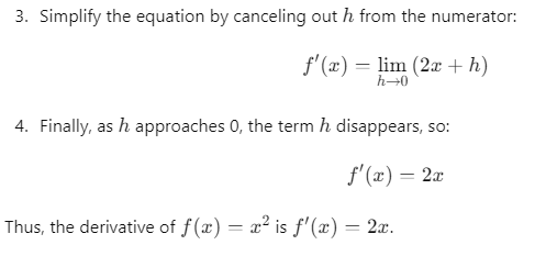
In calculus, a derivative tells us how a function f(x) changes as the input x changes. It measures the rate of change of the function.
![Derivative formula showing the rate of change of a function with respect to x, represented as f'(x) = lim(h→0) [f(x+h) - f(x)] / h.](https://emitechlogic.com/wp-content/uploads/2024/10/Derivative-Formulas.png)
The formula calculates the ratio of the change in f(x) to the change in x (which is h). As h gets smaller and approaches zero, this ratio becomes the instantaneous rate of change of the function.

Python Code Explanation
Now that we understand the math, let’s dive into the Python code that implements this.
Code Breakdown
Here’s the code snippet we used:
import numpy as np

# Define the function f(x) = x^2
def f(x):
    return x**2

# Define a function to calculate the derivative
def derivative(f, x):
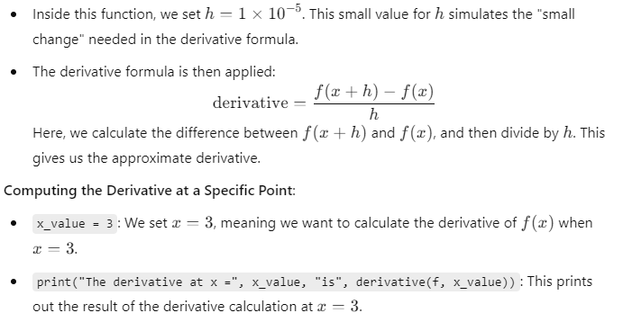
    h = 1e-5  # A very small change in x (h is close to 0)
    return (f(x + h) - f(x)) / h  # Apply the derivative formula

# Calculate the derivative at x = 3
x_value = 3
print("The derivative at x =", x_value, "is", derivative(f, x_value))
Explanation of Each Part
- Importing NumPy:
import numpy as np: We import the NumPy library. While it’s not directly needed here, it’s often used for more complex mathematical operations in data science.
- Defining the Function:
def f(x): return x**2: Here, we define the function f(x) = x^2. You can replace x^2 with any function you want to find the derivative for.
- Calculating the Derivative:
def derivative(f, x):: This is a function that computes the derivative of any given function f(x).
Code Output
If you run this code, the output will be:
The derivative at x = 3 is 6.000000000039306
This result is close to the exact derivative we calculated earlier using math, where we found that the derivative of f(x) = x^2 at x=3 is 6 since xf'(x) = 2x, and 2(3)=6.
Visualizing the Derivative
You can also visualize how the derivative works by plotting the function and its derivative. Here’s an additional code snippet to create a visual:
import numpy as np
import matplotlib.pyplot as plt

# Define the function f(x) = x^2
def f(x):
    return x**2

# Define a range of x values
x_values = np.linspace(-5, 5, 100)

# Calculate the y values for the function f(x) and its derivative
y_values = f(x_values)
derivative_values = 2 * x_values  # The derivative of f(x) = x^2 is 2x

# Plot the function and its derivative
plt.plot(x_values, y_values, label='f(x) = x^2')
plt.plot(x_values, derivative_values, label="f'(x) = 2x", linestyle='--')

# Adding labels and title
plt.xlabel('x')
plt.ylabel('y')
plt.title('Function and Derivative')

# Displaying legend and plot
plt.legend()
plt.grid(True)
plt.show()
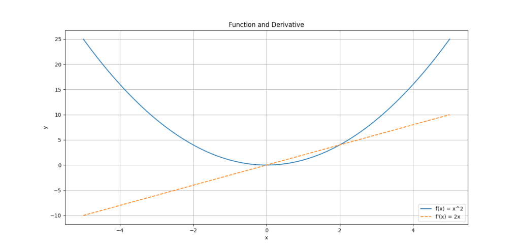
This will plot both the function f(x) = x^2 and its derivative f′(x)=2. You’ll notice that the slope (or rate of change) increases as x gets larger.
Basic Derivative Rules in Data Science
When working with Derivatives in Data Science, understanding the fundamental rules is essential. These rules help us deal with more complex functions, especially in machine learning when optimizing models. Let’s walk through three major rules — the Product Rule, Quotient Rule, and Chain Rule — that you’ll come across frequently.
1. Product Rule in Data Science
The Product Rule helps when you need to differentiate two functions that are multiplied together. This is common in data science, especially when dealing with feature interactions or cost functions in machine learning models that involve multiple variables working together.
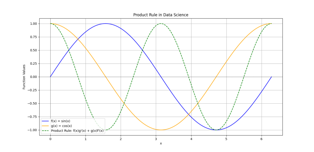
Explanation of the Plot:
- Blue Line: Represents f(x)=sin(x).
- Orange Line: Represents g(x)=cos(x).
- Green Dashed Line: Represents the derivative obtained using the product rule, calculated as f(x)g′(x)+g(x)f′(x).
This visualization helps to understand how the product rule operates in the context of these functions, emphasizing the changes in their combined behavior
Mathematical Explanation:
For two functions f(x) and g(x), the Product Rule states:

Data Science Context:
You are working on a regression model where two features (variables) interact with each other. For example, in a dataset predicting house prices, one feature could be the square footage of the house, and another could be the number of bedrooms. These two features together might affect the outcome in a multiplicative way. In such cases, you’d apply the Product Rule when calculating gradients to optimize your model.
Python Code Example:
Let’s use SymPy, a Python library for symbolic mathematics, to apply the Product Rule:
import sympy as sp

# Define the variable and functions
x = sp.symbols('x')
f = x**2  # f(x) = x^2
g = sp.sin(x)  # g(x) = sin(x)

# Apply the product rule
product_rule = sp.diff(f * g, x)
print(product_rule)
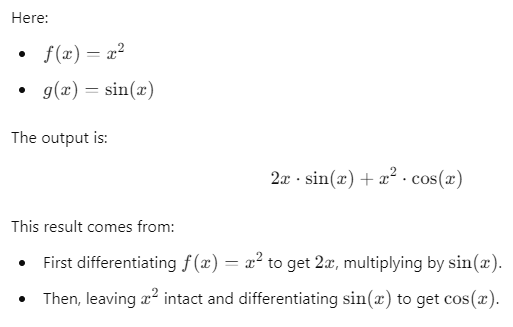
Real-World Application: In gradient descent, the Product Rule helps compute the gradient for terms that involve feature interaction in machine learning models. It ensures that both parts of the function are considered during optimization, improving the accuracy of the model.
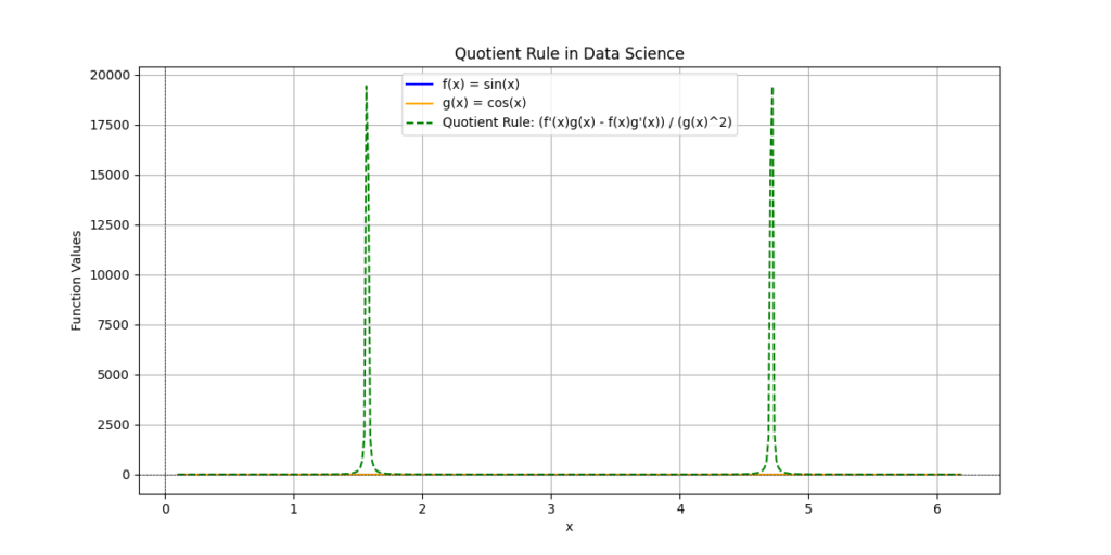
2. Quotient Rule in Data Science
The Quotient Rule is used when you are differentiating a ratio of two functions. In data science, this rule is handy when calculating the ratio of two variables or when dealing with error metrics or likelihood functions in machine learning.
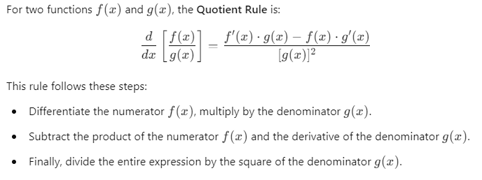
Mathematical Explanation:
For two functions f(x) and g(x), the Quotient Rule is:
Python Code Example:
Let’s implement this using SymPy:
# Define functions for the quotient rule
f = x**2  # f(x) = x^2
g = sp.exp(x)  # g(x) = exp(x)

# Apply the quotient rule
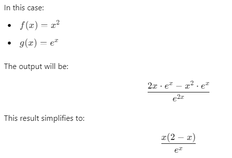
quotient_rule = sp.diff(f / g, x)
print(quotient_rule)
Data Science Context:
When you’re working on logistic regression or maximum likelihood estimation (MLE), you might need to compute the gradient of a likelihood function. Often, these functions are expressed as a ratio, making the Quotient Rule essential in finding the correct gradient during optimization.
3. Chain Rule in Data Science
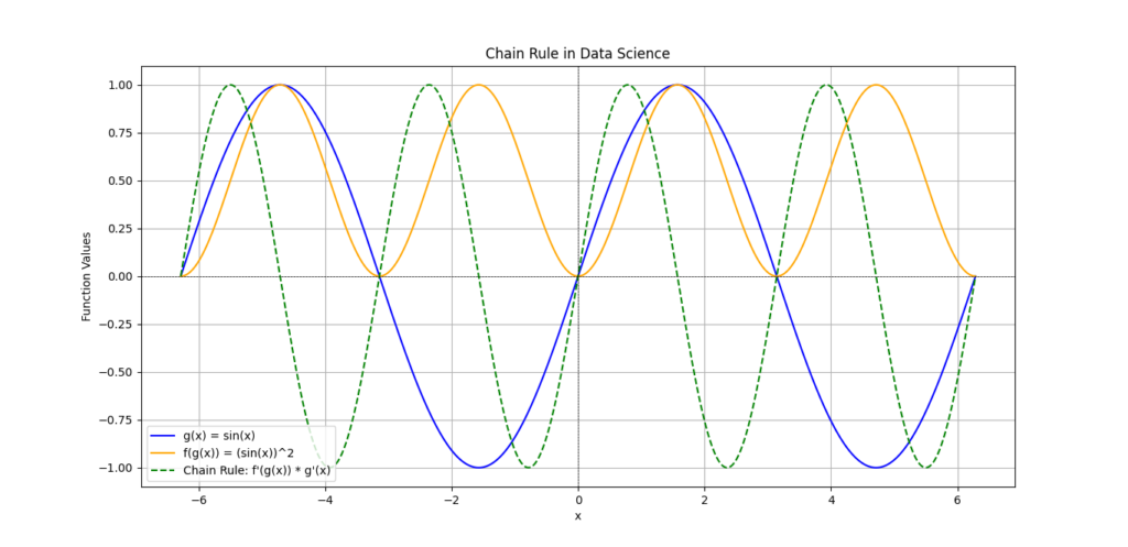
The Chain Rule is extremely important in data science, especially in deep learning and neural networks. It helps when differentiating composite functions — functions inside other functions. The Chain Rule is critical for calculating gradients through multiple layers in a neural network, a process known as backpropagation.
Mathematical Explanation:
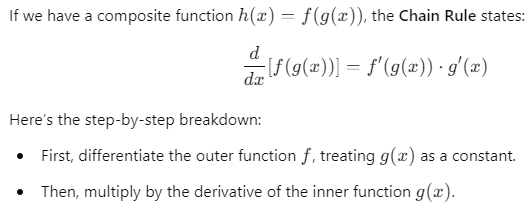
If we have a composite function h(x)=f(g(x)), the Chain Rule states:
Python Code Example:
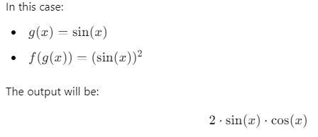
Let’s see an example of the Chain Rule in Python:
# Define functions for the chain rule
g = sp.sin(x)  # Inner function g(x) = sin(x)
f = g**2  # Composite function f(g(x)) = (sin(x))^2

# Apply the chain rule
chain_rule = sp.diff(f, x)
print(chain_rule)
Data Science Context:
In deep learning, the Chain Rule is important for backpropagation. Neural networks consist of layers of functions that are composed together. When training the network, we compute the gradient of the loss function with respect to each weight by applying the Chain Rule across each layer. This allows the network to update its weights correctly and minimize errors through gradient descent.
Summary of Derivative Rules
Here’s a tabulated summary to make these rules clearer:

Understanding Gradient Descent
In the world of machine learning, gradient descent plays a crucial role. It is a powerful optimization algorithm used to minimize the cost function in various models. The cost function quantifies how well a model is performing. The goal is to reduce this cost, which is where gradient descent comes into play. This article will explain the concept of gradient descent, its importance, and how Derivatives in Data Science are utilized in this process.
What is Gradient Descent?
Gradient descent is an iterative optimization algorithm. It aims to find the minimum value of a function, often used in machine learning to minimize the error between the predicted values and the actual data. The algorithm starts with an initial guess for the parameters (often random) and then continuously adjusts them to minimize the cost function.
Here’s a step-by-step breakdown of how gradient descent works:
- Initialize Parameters: Start with random values for the parameters (weights) of your model.
- Calculate the Cost: Compute the cost function J(θ)J(\theta)J(θ) to understand how well the model is performing.
- Compute the Gradient: Use derivatives to calculate the gradient. This tells you the direction in which the cost function increases.
- Update the Parameters: Adjust the parameters in the opposite direction of the gradient to minimize the cost.
- Iterate: Repeat steps 2 to 4 until the cost function converges to a minimum value or the changes become negligible.
Importance of Derivatives in Gradient Descent
Derivatives are fundamental in calculating both the direction and magnitude of the descent in gradient descent. The gradient provides a vector of partial derivatives, indicating how much the cost function J(θ)J(\theta)J(θ) will change with respect to each parameter.
- Direction: The sign of the derivative tells you whether to increase or decrease the parameter. If the derivative is positive, you will want to move in the negative direction to reduce the cost. Conversely, if the derivative is negative, you should move in the positive direction.
- Magnitude: The size of the gradient determines how much to change the parameter. A large gradient indicates that a significant adjustment is needed, while a small gradient suggests a more subtle adjustment.
The formula for updating the parameters can be expressed as:
θ=θ−α⋅∇J(θ)
Where:
- θ represents the parameters,
- α is the learning rate (a small constant that determines how big each update step is),
- ∇J(θ) is the gradient of the cost function.
Example of Gradient Descent in Machine Learning
Let’s take a closer look at how gradient descent can be applied in a simple linear regression example.
Linear Regression Example
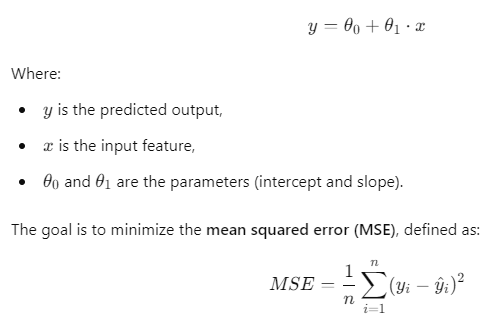
In linear regression, the relationship between input features and output predictions can be expressed as:
Where:
- n is the number of data points,
- y_i is the actual value,
- y^i is the predicted value.
Implementing Gradient Descent in Python
Here’s how you could implement gradient descent for linear regression using Python:
import numpy as np

# Define the mean squared error function
def compute_cost(X, y, theta):
    m = len(y)
    return (1 / (2 * m)) * np.sum((X.dot(theta) - y) ** 2)

# Gradient descent function
def gradient_descent(X, y, theta, learning_rate, iterations):
    m = len(y)
    for i in range(iterations):
        # Calculate the gradient
        gradient = (1 / m) * X.T.dot(X.dot(theta) - y)
        # Update parameters
        theta = theta - learning_rate * gradient
    return theta

# Sample data
X = np.array([[1, 1], [1, 2], [1, 3]])  # Including the intercept term
y = np.array([1, 2, 3])  # Actual outputs
theta = np.array([0.0, 0.0])  # Initial parameters

# Run gradient descent
theta_optimized = gradient_descent(X, y, theta, learning_rate=0.01, iterations=1000)
print("Optimized Parameters:", theta_optimized)
Visualizing Gradient Descent
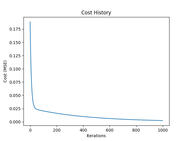
Visualizing the optimization process can help understand how gradient descent works. Below is a simple way to visualize the updates to the parameters:
import numpy as np
import matplotlib.pyplot as plt

# Function to compute cost (Mean Squared Error)
def compute_cost(X, y, theta):
    m = len(y)
    predictions = X.dot(theta)
    cost = (1 / (2 * m)) * np.sum(np.square(predictions - y))
    return cost

# Function to plot cost history
def plot_cost_history(cost_history):
    plt.plot(cost_history)
    plt.xlabel('Iterations')
    plt.ylabel('Cost (MSE)')
    plt.title('Cost History')
    plt.show()

# Function to perform gradient descent and track cost history
def gradient_descent_with_history(X, y, theta, learning_rate, iterations):
    m = len(y)
    cost_history = np.zeros(iterations)

    for i in range(iterations):
        gradient = (1 / m) * X.T.dot(X.dot(theta) - y)
        theta = theta - learning_rate * gradient
        cost_history[i] = compute_cost(X, y, theta)

    return theta, cost_history

# Sample data (replace with your own data)
# Define input features (X) and output labels (y)
# Here, we create a simple linear dataset for demonstration
X = np.array([[1, 1], [1, 2], [1, 3]])  # Add a column of ones for the intercept
y = np.array([1, 2, 3])                   # Output values
theta = np.array([0.5, 0.5])              # Initial guess for theta

# Run gradient descent with cost tracking
theta_optimized, cost_history = gradient_descent_with_history(X, y, theta, learning_rate=0.01, iterations=1000)

# Plot the cost history
plot_cost_history(cost_history)
Summary of Gradient Descent
In summary, gradient descent is an essential algorithm in machine learning. By iteratively updating model parameters using the gradient of the cost function, the algorithm efficiently finds the optimal values that minimize error.
Key Points:
Visualizations help understand the optimization process and how the cost decreases over iterations.
Gradient Descent is used to minimize the cost function in machine learning models.
Derivatives play a crucial role in determining both the direction and magnitude of parameter updates.
How Derivatives Help Minimize Cost Functions
In the realm of machine learning, optimizing a model’s performance is essential. One of the key ways to achieve this is through the minimization of cost functions. The cost function quantifies how well a model is performing by measuring the difference between the predicted values and the actual values. In this context, Derivatives in Data Science play a crucial role in guiding the optimization process.
This article will explore how derivatives are used to minimize cost functions in machine learning models, focusing on linear regression as a primary example. Let’s break down the concepts step by step.
Understanding Cost Functions
A cost function is a mathematical expression that represents the error of a model. It calculates how far off the predictions are from the actual outcomes. The goal in machine learning is to minimize this error, leading to more accurate predictions.
- Common Cost Functions:
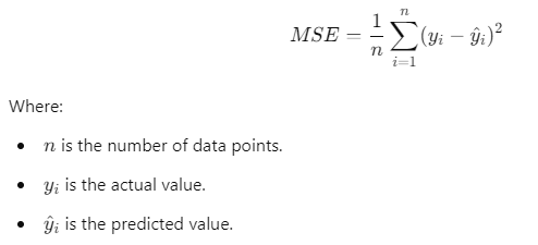
- Mean Squared Error (MSE): Measures the average of the squares of the errors between predicted and actual values.
- Cross-Entropy Loss: Often used in classification problems to evaluate the performance of a model whose output is a probability value between 0 and 1.
For linear regression, the Mean Squared Error (MSE) is typically used and can be defined mathematically as:
The Role of Derivatives in Cost Function Optimization
Derivatives are essential in understanding how the cost function changes with respect to the model parameters. By calculating the derivative of the cost function, you can determine how to adjust the parameters to reduce the error. This process is often referred to as gradient descent, a fundamental algorithm in machine learning.
- Finding the Gradient: The derivative of the cost function gives you the gradient, which indicates the direction and steepness of the cost function.
- Direction of Change:
- If the derivative is positive, it suggests that increasing the parameter will lead to an increase in cost. Thus, you should decrease the parameter to minimize the cost.
- If the derivative is negative, increasing the parameter will decrease the cost. Therefore, an increase is warranted.
- Adjusting Parameters: The parameters are updated based on the gradient to minimize the cost function.
The formula for updating the parameters θ\thetaθ can be expressed as:
θ=θ−α⋅∇J(θ)
Where:
- α is the learning rate.
- ∇J(θ) is the gradient of the cost function.
Example: Linear Regression Using Derivatives in Data Science
Let’s illustrate how derivatives help minimize the cost function in a linear regression model.
- Model Definition: In linear regression, the relationship between the input x and the output y is defined as:

Implementing Gradient Descent in Python
Here’s how you can implement the gradient descent algorithm for linear regression using Python, focusing on the use of derivatives:
import numpy as np

# Function to compute the mean squared error
def compute_cost(X, y, theta):
    m = len(y)
    return (1 / (2 * m)) * np.sum((X.dot(theta) - y) ** 2)

# Gradient descent algorithm
def gradient_descent(X, y, theta, learning_rate, iterations):
    m = len(y)
    for i in range(iterations):
        # Calculate the gradient
        gradient = (1 / m) * X.T.dot(X.dot(theta) - y)
        # Update parameters
        theta = theta - learning_rate * gradient
    return theta

# Sample data
X = np.array([[1, 1], [1, 2], [1, 3]])  # Including the intercept term
y = np.array([1, 2, 3])  # Actual outputs
theta = np.array([0.0, 0.0])  # Initial parameters

# Running gradient descent
theta_optimized = gradient_descent(X, y, theta, learning_rate=0.01, iterations=1000)
print("Optimized Parameters:", theta_optimized)
Output:
Optimized Parameters: [0.11071521 0.95129619]
Explanation of the Code
- Data Initialization: The data X includes an intercept term (1s) for the bias, and yyy holds the actual outputs.
- Cost Function Calculation: The
compute_costfunction calculates the MSE to evaluate the model’s performance. - Gradient Descent Implementation: The
gradient_descentfunction:- Calculates the gradient of the cost function.
- Updates the parameters θ\thetaθ based on the gradient and learning rate.
- Final Output: After running for a specified number of iterations, the optimized parameters are printed. These parameters represent the slope and intercept that minimize the cost function.
Must Read
- Why sorted() Is Safer Than list.sort() in Production Python Systems
- Monotonic Sequence in Python: 7 Practical Methods With Edge Cases, Interview Tips, and Performance Analysis
- How to Check if Dictionary Values Are Sorted in Python
- Check If a Tuple Is Sorted in Python — 5 Methods Explained
- How to Check If a List Is Sorted in Python (Without Using sort()) – 5 Efficient Methods
Derivatives in Neural Networks
Derivatives and Backpropagation
In neural networks, one of the most important processes is backpropagation. This method, which uses partial derivatives to adjust the weights, is what allows neural networks to learn from data. By breaking down backpropagation into easy-to-understand parts, we can see how Derivatives in Data Science play a central role in making machine learning models smarter over time.
What is Backpropagation?
Backpropagation (short for “backward propagation of errors”) is an algorithm used in training artificial neural networks. It works by calculating the error in the output layer and then distributing that error backward through the network to update the weights. These weight adjustments are based on the partial derivatives of the error with respect to each weight. This way, the model learns by minimizing its prediction error.
The key steps in backpropagation:
- Feedforward phase: The input data is passed through the network layer by layer until it reaches the output.
- Error calculation: The difference (error) between the predicted and actual output is calculated using a cost function.
- Backward phase: The algorithm uses the error to adjust the weights by calculating partial derivatives of the cost function with respect to each weight.
- Weight update: The weights are updated using gradient descent, allowing the model to improve its predictions over time.
Backpropagation’s reliance on derivatives makes it essential for deep learning and machine learning models to function effectively. The use of partial derivatives in machine learning allows backpropagation to understand how changes in weights affect the overall error, and it directs the model on how to improve itself.
How Partial Derivatives Work in Neural Networks
Let’s say we have a simple neural network with two layers: an input layer and an output layer. The key part of training the network is to calculate how each weight contributes to the overall error. This is done using partial derivatives.
Imagine the cost function J as a function of multiple weights w_1, w_2, w_3, etc. To understand how the error changes with each weight, we calculate the partial derivative of J with respect to each weight:

These partial derivatives tell us how much the cost function changes when each specific weight changes. This helps the neural network determine which weights need more adjustment to reduce the overall error during the training process.
Derivatives in Backpropagation: Step-by-Step Breakdown
- Input Layer: The network starts by taking the input data and passing it through each layer of the neural network during the forward pass.
- Output Layer: The network makes predictions based on the input data. The predictions are compared to the actual outputs (labels), and the error (or cost) is calculated using a cost function like mean squared error (MSE) or cross-entropy.
- Calculating Derivatives: For each weight, the partial derivative of the cost function with respect to the weight is calculated. This tells us how much influence each weight has on the overall error.
- Updating Weights: Once the partial derivatives are known, gradient descent is used to update the weights. The weight update rule looks like this:

This process is repeated for multiple iterations until the model’s error reaches a minimum.
Example: Derivatives in Neural Network Training
Let’s walk through a basic example to see how derivatives work during neural network training. We will create a simple neural network and use backpropagation to adjust the weights.
Python Code Example: Training a Simple Neural Network with Derivatives
import numpy as np

# Sigmoid activation function and its derivative
def sigmoid(x):
    return 1 / (1 + np.exp(-x))

def sigmoid_derivative(x):
    return x * (1 - x)

# Training data
X = np.array([[0, 0], [0, 1], [1, 0], [1, 1]])  # Input data (XOR problem)
y = np.array([[0], [1], [1], [0]])  # Expected output

# Initialize weights randomly
np.random.seed(1)
weights_input_hidden = np.random.rand(2, 2)
weights_hidden_output = np.random.rand(2, 1)

# Learning rate
learning_rate = 0.1

# Training the network
for epoch in range(10000):  # Training for 10,000 iterations
    # Forward pass
    hidden_layer_input = np.dot(X, weights_input_hidden)
    hidden_layer_output = sigmoid(hidden_layer_input)

    final_layer_input = np.dot(hidden_layer_output, weights_hidden_output)
    final_layer_output = sigmoid(final_layer_input)

    # Calculate error
    error = y - final_layer_output

    # Backpropagation
    d_output = error * sigmoid_derivative(final_layer_output)

    error_hidden_layer = d_output.dot(weights_hidden_output.T)
    d_hidden_layer = error_hidden_layer * sigmoid_derivative(hidden_layer_output)

    # Update weights
    weights_hidden_output += hidden_layer_output.T.dot(d_output) * learning_rate
    weights_input_hidden += X.T.dot(d_hidden_layer) * learning_rate

# Print final output
print("Trained output after 10,000 iterations:")
print(final_layer_output)
Code Breakdown:
- Sigmoid Function: We use the sigmoid activation function, which outputs values between 0 and 1. Its derivative helps us calculate how much to adjust the weights.
- Forward Pass: The input data X is passed through the network, and the output is calculated at each layer. In this case, the network is designed to solve the XOR problem.
- Error Calculation: We calculate the difference between the network’s predicted output and the expected output yyy. This difference is the error that will be used to adjust the weights.
- Backpropagation: Using the sigmoid derivative, we calculate the partial derivatives of the error with respect to each weight and adjust them accordingly.
- Updating Weights: The weights are updated using gradient descent based on the calculated partial derivatives. The process is repeated for several iterations (10,000 in this case) to minimize the error.
Applications of Derivatives in Data Science
Derivatives in Linear and Logistic Regression – Derivatives in Data Science
Understanding Derivative-Based Optimization
In the realm of machine learning, derivatives play a critical role in optimizing models like linear regression and logistic regression. By using derivatives, we can effectively minimize the error between predicted and actual values, leading to improved model performance.
How Derivatives Help Optimize Linear Regression
Linear regression aims to find the best-fitting line through a set of data points. This line is represented by the equation:
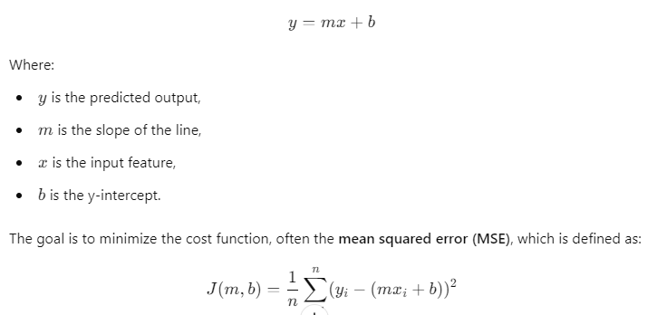
Where:
- J is the cost function,
- n is the number of data points,
- y_i is the actual output,
- x_i is the input feature.
To find the optimal values of mmm and bbb, we calculate the derivatives of the cost function with respect to each parameter. The gradients tell us the direction and magnitude to adjust mmm and bbb to minimize the error.
Step-by-Step Explanation of Calculating the Gradient for Linear Regression
- Calculate the Cost Function: Start with the mean squared error function J(m,b).
- Find the Derivatives:
- Derivative with respect to m:
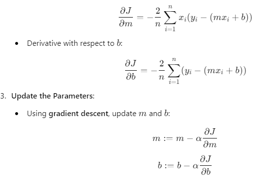
Where α is the learning rate, controlling how much we adjust the weights at each step.
- Iterate: Repeat the process until the cost function converges to a minimum value.
Derivatives in Logistic Regression
Logistic regression is used for binary classification tasks. The model predicts the probability that an instance belongs to a particular class. The logistic function (or sigmoid function) is defined as:
![Logistic regression model for binary classification: Logistic function (sigmoid function): 𝜎 ( 𝑧 ) = 1 1 + 𝑒 − 𝑧 σ(z)= 1+e −z 1 Where 𝑧 = 𝑚 𝑥 + 𝑏 z=mx+b Cost function for logistic regression: 𝐽 ( 𝑚 , 𝑏 ) = − 1 𝑛 ∑ 𝑖 = 1 𝑛 [ 𝑦 𝑖 log ( 𝜎 ( 𝑧 𝑖 ) ) + ( 1 − 𝑦 𝑖 ) log ( 1 − 𝜎 ( 𝑧 𝑖 ) ) ] J(m,b)=− n 1 ∑ i=1 n [y i log(σ(z i ))+(1−y i )log(1−σ(z i ))]](https://emitechlogic.com/wp-content/uploads/2024/10/Logistic-regression.png)
Calculating the Gradient for Logistic Regression
- Calculate the Cost Function: Use the logistic cost function J(m,b).
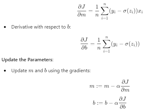
- Find the Derivatives:
- Derivative with respect to m:
Key Points
- Derivatives help optimize linear and logistic regression models.
- The gradients indicate the direction to adjust the model parameters to minimize the error.
- The process involves calculating cost functions, finding derivatives, and updating parameters iteratively.
Derivatives in Clustering Algorithms
Using Derivatives in Clustering Algorithms like K-Means
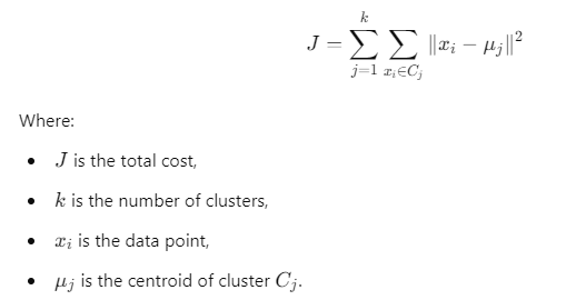
Clustering is another important application of derivatives in machine learning. The K-means algorithm is a popular clustering technique used to partition data into kkk distinct clusters. The primary goal is to minimize the distance between the data points and their respective cluster centroids.
How K-Means Uses Derivatives in Data Science
- Initialize Centroids: Choose kkk initial centroids randomly.
- Assign Clusters: Each data point is assigned to the nearest centroid.
- Update Centroids: The centroids are recalculated as the mean of the data points assigned to each cluster.
- Minimize the Cost Function: The cost function for K-means is defined as:
Using Derivatives in Data Science to Find Optimal Centroids
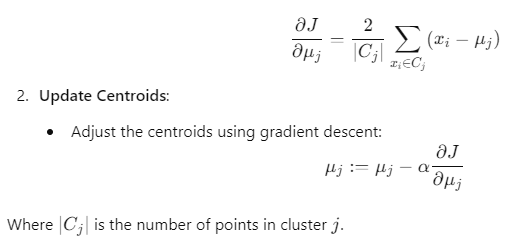
To find the optimal centroids, we calculate the derivative of the cost function with respect to each centroid:
- Calculate the Derivative:
- For each centroid, we find the derivative of the cost function J:
Code Example: Centroid Adjustment Using Derivatives in Data Science
Here’s a simple implementation of the K-means algorithm demonstrating how derivatives are used to adjust centroids:
import numpy as np

# Generate random data
np.random.seed(0)
data = np.random.rand(100, 2)

# Number of clusters
k = 3
centroids = data[np.random.choice(data.shape[0], k, replace=False)]

def kmeans(data, centroids, iterations=100):
    for _ in range(iterations):
        # Assign clusters
        distances = np.linalg.norm(data[:, np.newaxis] - centroids, axis=2)
        labels = np.argmin(distances, axis=1)

        # Update centroids
        for j in range(k):
            if len(data[labels == j]) > 0:
                centroids[j] = np.mean(data[labels == j], axis=0)
    return centroids, labels

final_centroids, final_labels = kmeans(data, centroids)

print("Final centroids:")
print(final_centroids)
Code Breakdown
- Random Data Generation: We create a simple dataset of 100 points in two dimensions.
- Centroid Initialization: The centroids are initialized randomly from the data points.
- K-means Function: The function iteratively assigns each data point to the nearest centroid and updates the centroids based on the mean of the assigned points.
Key Takeaways:
- Derivatives help optimize regression models and clustering algorithms.
- In linear regression, they guide parameter updates based on minimizing the mean squared error.
- In logistic regression, they help adjust parameters to classify data accurately.
- In K-means, derivatives are used to find optimal centroids that minimize distances to data points.
By grasping these concepts, you will be better equipped to implement and optimize machine learning models using Derivatives in Data Science.
Advanced Topics: Second Derivatives in Data Science and Convex Optimization
Second Derivatives: What Are They?
Understanding Second Derivatives in Data Science
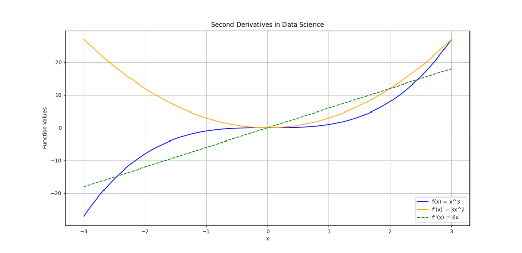
When we study Derivatives in Data Science, we typically begin with first derivatives. The first derivative of a function measures the rate of change of the function at a specific point. In simpler terms, it tells us how steep the function is or whether it is increasing or decreasing at that point.
However, the second derivative provides even deeper insights. It is the derivative of the first derivative, effectively measuring the rate of change of the rate of change. This means that the second derivative can tell us how the slope of a function is changing. Here’s a brief breakdown:
- First Derivative (f′(x)): Indicates the slope or direction of a function (increasing or decreasing).
- Second Derivative (f′′(x)): Reveals the concavity of the function:
- Positive Second Derivative: The function is concave up (like a cup) and the slope is increasing.
- Negative Second Derivative: The function is concave down (like a cap) and the slope is decreasing.
Introducing the Hessian Matrix
The Hessian matrix is a vital tool in multivariable calculus that contains all the second-order partial derivatives of a function. It is particularly useful in optimization problems involving multiple variables.
For a function f(x1,x2,…,xn), the Hessian matrix H is defined as:
![The Hessian matrix, represented as: 𝐻 = [ ∂ 2 𝑓 ∂ 𝑥 1 2 ∂ 2 𝑓 ∂ 𝑥 1 ∂ 𝑥 2 ⋯ ∂ 2 𝑓 ∂ 𝑥 1 ∂ 𝑥 𝑛 ∂ 2 𝑓 ∂ 𝑥 2 ∂ 𝑥 1 ∂ 2 𝑓 ∂ 𝑥 2 2 ⋯ ∂ 2 𝑓 ∂ 𝑥 2 ∂ 𝑥 𝑛 ⋮ ⋮ ⋱ ⋮ ∂ 2 𝑓 ∂ 𝑥 𝑛 ∂ 𝑥 1 ∂ 2 𝑓 ∂ 𝑥 𝑛 ∂ 𝑥 2 ⋯ ∂ 2 𝑓 ∂ 𝑥 𝑛 2 ] H= ∂x 1 2 ∂ 2 f ∂x 2 ∂x 1 ∂ 2 f ⋮ ∂x n ∂x 1 ∂ 2 f ∂x 1 ∂x 2 ∂ 2 f ∂x 2 2 ∂ 2 f ⋮ ∂x n ∂x 2 ∂ 2 f ⋯ ⋯ ⋱ ⋯ ∂x 1 ∂x n ∂ 2 f ∂x 2 ∂x n ∂ 2 f ⋮ ∂x n 2 ∂ 2 f The Hessian matrix is used to analyze critical points of a function based on its second derivatives.](https://emitechlogic.com/wp-content/uploads/2024/10/Hessian-matrix.png)
The Hessian matrix helps identify the nature of critical points (where the first derivative is zero) in a function. For example:
- If the Hessian is positive definite at a critical point, that point is a local minimum.
- If it is negative definite, the point is a local maximum.
- If the Hessian is indefinite, the critical point is a saddle point.
How Second Derivatives Are Used in Optimization
The Role of Second Derivatives in Optimization
In optimization, second Derivatives in Data Science play a crucial role. They can fine-tune models by identifying local minima and maxima. This capability can lead to more effective training of machine learning models and faster convergence.
Identifying Minima and Maxima
When training models, particularly in machine learning, understanding the nature of the loss function is essential. The goal is often to minimize this loss function. Here’s how second derivatives help:
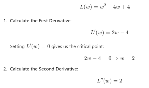
- Finding Critical Points: The first derivative is set to zero to find critical points.
- Using the Hessian: The second derivative (or Hessian matrix) is then analyzed at these critical points:
- Positive values indicate a local minimum.
- Negative values indicate a local maximum.
- A mix of positive and negative values indicates a saddle point.
This analysis is crucial for methods like Newton’s method, which uses second derivatives to refine estimates of the minimum more rapidly.
Example: Using Second Derivatives in Convex Optimization
Let’s consider a simple example where we use second derivatives for optimization in machine learning. The objective is to minimize a convex function represented by the loss function L(w):
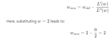
Code Example: Using Hessian in Python
Here’s a simple code snippet demonstrating how second derivatives can be used in optimization:
import numpy as np

# Define the loss function
def loss_function(w):
    return w**2 - 4*w + 4

# Define the first derivative
def first_derivative(w):
    return 2*w - 4

# Define the second derivative
def second_derivative():
    return 2

# Using Newton's method for optimization
def newtons_method(w_init, tolerance=1e-5, max_iter=100):
    w = w_init
    for _ in range(max_iter):
        grad = first_derivative(w)
        hess = second_derivative()
        if abs(grad) < tolerance:  # Check for convergence
            break
        w -= grad / hess
    return w

# Initial guess
initial_w = 0.0
optimal_w = newtons_method(initial_w)
print("Optimal value of w:", optimal_w)
Code Breakdown
- Loss Function: A simple quadratic loss function is defined.
- Derivatives: The first and second derivatives are calculated.
- Newton’s Method: This method iteratively refines the estimate of www using the derivatives.
Key Takeaways:
- Second derivatives provide insights into the rate of change of the first derivative.
- The Hessian matrix contains second-order partial derivatives, aiding in optimization.
- Analyzing second derivatives helps identify local minima, maxima, and saddle points.
- Techniques like Newton’s method utilize second derivatives for rapid convergence.
By mastering these concepts, you will have a powerful toolset for applying Derivatives in Data Science, making your models more efficient and effective.
Latest Advancements in Derivatives for Data Science
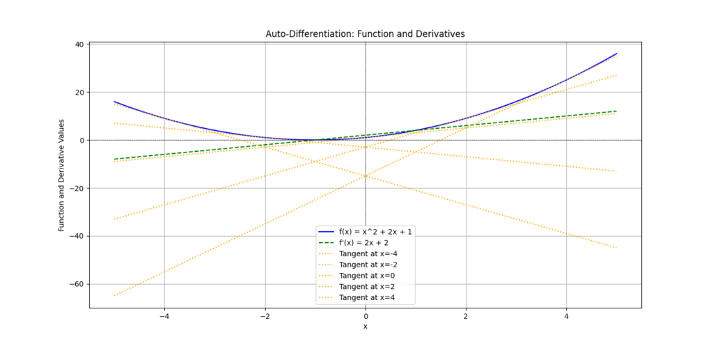
What is Auto-Differentiation?
Auto-differentiation is a powerful technique that automates the process of calculating derivatives. In machine learning, it plays a crucial role in optimizing models, as derivatives are essential for updating model parameters during training. The ability to compute derivatives efficiently can significantly speed up the training process and improve the performance of machine learning algorithms.
Unlike numerical differentiation, which approximates derivatives using finite differences, or symbolic differentiation, which derives mathematical expressions, automatic differentiation achieves both accuracy and efficiency. It systematically applies the chain rule of calculus to compute derivatives accurately for complex functions.
This method becomes especially valuable in deep learning, where models can consist of many layers and intricate operations. Auto-differentiation simplifies complex derivative calculations, allowing researchers and practitioners to focus on designing and fine-tuning their models instead of worrying about the math behind the scenes.
How Auto-Differentiation Simplifies Complex Derivative Calculations
The process of automatic differentiation can be understood through two main modes:
- Forward Mode: This mode computes derivatives alongside the evaluation of the function. It is particularly effective when the function has a small number of outputs and many inputs. For each variable, the derivative is propagated forward through the computational graph.
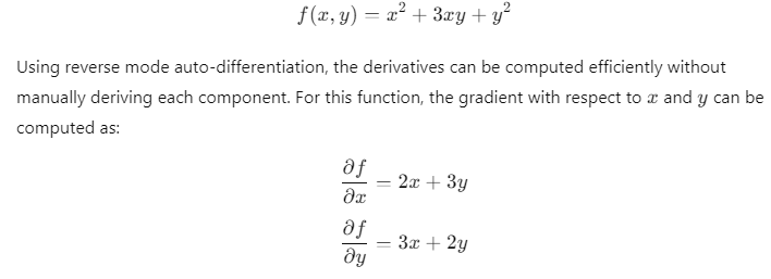
- Reverse Mode: This mode is more commonly used in machine learning frameworks. It calculates derivatives in a backward pass after the function is evaluated. This approach is ideal when the function has many outputs and fewer inputs, which is often the case in deep learning models. The gradients of the output with respect to the inputs are computed efficiently.
To illustrate, consider the following simple function:
Benefits of Automatic Differentiation
- Efficiency: Reduces computation time compared to numerical differentiation.
- Accuracy: Provides exact derivatives without approximations.
- Simplicity: Frees data scientists from manual derivative calculations, allowing them to focus on model architecture.
Tools for Automatic Differentiation in Data Science
Overview of Tools Like TensorFlow and PyTorch
Several popular tools in data science leverage automatic differentiation to enhance model training and optimization. Two of the most widely used frameworks are TensorFlow and PyTorch. Both frameworks have built-in support for auto-differentiation, making them ideal choices for developing and training machine learning models.
TensorFlow Automatic Differentiation
In TensorFlow, the automatic differentiation feature is integrated into the tf.GradientTape context manager. This approach allows for the recording of operations for automatic differentiation.
Here’s a simple example:
import tensorflow as tf

# Define a function
def function(x):
    return x**2 + 3*x + 5

# Using GradientTape for automatic differentiation
x = tf.Variable(2.0)
with tf.GradientTape() as tape:
    y = function(x)

# Calculate the derivative
dy_dx = tape.gradient(y, x)
print("The derivative at x = 2.0 is:", dy_dx.numpy())
In this example, TensorFlow automatically computes the derivative of the function f(x) at x=2.0.
PyTorch Autograd
PyTorch offers a similar feature through its autograd module. This module records operations on tensors to automatically compute gradients during backpropagation.
Here’s how it works in PyTorch:
import torch

# Define a function
def function(x):
    return x**2 + 3*x + 5

# Create a tensor with gradient tracking
x = torch.tensor(2.0, requires_grad=True)
y = function(x)

# Calculate the derivative
y.backward()
print("The derivative at x = 2.0 is:", x.grad.item())
In this code snippet, the .backward() method computes the derivative of the function at x=2.0x = 2.0x=2.0 using automatic differentiation.
How These Tools Speed Up Model Training and Optimization
Using automatic differentiation significantly accelerates model training for several reasons:
- Reduced Coding Complexity: By automatically calculating derivatives, developers save time and reduce the risk of errors in manual calculations.
- Faster Experimentation: Data scientists can quickly prototype and test new ideas without being bogged down by derivative calculations.
- Optimized Resource Usage: Efficient calculations allow for larger models and datasets to be handled within reasonable time frames.
Summary of Benefits of Automatic Differentiation Tools
| Benefit | Description |
|---|---|
| Efficiency | Quick computation of gradients speeds up model training. |
| Accuracy | Provides precise derivatives for complex functions. |
| User-Friendly | Simplifies coding by automating derivative calculations. |
| Enhanced Experimentation | Allows for rapid testing of new model architectures and ideas. |
In summary, automatic differentiation is a game-changer in machine learning and data science. It automates the process of calculating derivatives, which simplifies the development of models. By using tools like TensorFlow and PyTorch, practitioners can leverage this technique to enhance their workflow, leading to faster and more effective model training.
Common Derivative Mistakes in Data Science
Ignoring Learning Rate Adjustments
Risks of Using the Wrong Learning Rate with Gradient Descent
When training machine learning models, the learning rate plays a crucial role in the optimization process, especially when using gradient descent. The learning rate determines how much to change the model’s parameters in response to the calculated gradients. Setting an inappropriate learning rate can lead to significant issues during training.
Understanding Learning Rate Issues
- Too High of a Learning Rate: If the learning rate is set too high, the model can overshoot the minimum of the loss function. This results in divergence, where the cost increases instead of decreasing. In such cases, the optimization process might oscillate wildly or fail altogether. For example, when trying to find the minimum point of a simple quadratic function, a high learning rate can lead to jumps over the minimum, preventing convergence.
- Too Low of a Learning Rate: Conversely, if the learning rate is too low, the optimization process becomes painfully slow. The model will make tiny adjustments to its parameters, leading to a prolonged training time. In some cases, it may get stuck in a local minimum, failing to explore potentially better solutions elsewhere.
Here’s a basic illustration of how the learning rate affects gradient descent:
- High Learning Rate:
- Outcome: Divergence
- Graph Behavior: The cost function fluctuates without settling.
- Low Learning Rate:
- Outcome: Slow Convergence
- Graph Behavior: The cost function decreases very slowly.
Example of Learning Rate in Action
In Python, using libraries like TensorFlow or PyTorch, one can easily visualize how different learning rates affect the training of a model. Here’s a simplified example using PyTorch:
import torch
import torch.nn as nn
import torch.optim as optim

# Sample data
x = torch.tensor([[1.0], [2.0], [3.0], [4.0]])
y = torch.tensor([[2.0], [3.0], [4.0], [5.0]])

# Simple linear model
model = nn.Linear(1, 1)

# Different learning rates
learning_rates = [0.1, 1.0, 10.0]

for lr in learning_rates:
    optimizer = optim.SGD(model.parameters(), lr=lr)
    criterion = nn.MSELoss()

    # Training loop
    for epoch in range(100):
        model.train()
        optimizer.zero_grad()
        output = model(x)
        loss = criterion(output, y)
        loss.backward()
        optimizer.step()

    print(f"Final loss with learning rate {lr}: {loss.item()}")
In this code snippet, different learning rates are applied to the same linear model. The final loss can highlight how a high learning rate might fail to minimize loss effectively compared to a more appropriate one.
Using the correct learning rate is essential for effective optimization in machine learning. An inappropriate learning rate can lead to slow convergence or divergence, undermining the entire training process. Understanding these risks is critical for data scientists who want to achieve the best results. Incorporating the knowledge of derivatives in calculus for data science can aid in selecting and adjusting the learning rate appropriately.
Misinterpreting Second Derivatives
Common Second Derivative Mistakes
Second Derivatives in Data Science, represented in the Hessian matrix, provide valuable information about the curvature of the loss function. However, misinterpreting these derivatives can lead to errors in model adjustments. It is essential to understand the role of second derivatives in optimization to avoid common pitfalls.
Importance of Second Derivatives in Optimization
- Identifying Curvature: The second derivative indicates how the slope of the function changes. Positive second derivatives indicate a local minimum, while negative ones indicate a local maximum. This information is critical when determining how to adjust model parameters effectively.
- Using the Hessian Matrix: The Hessian matrix is a square matrix of second-order mixed partial derivatives of a scalar-valued function. It provides insights into the local curvature of the loss function. When training a model, the Hessian can guide how much to adjust the parameters based on the curvature.
For example, if the Hessian is positive definite, the point is a local minimum, and small adjustments can be made confidently. If it is negative definite, the point is a local maximum, and adjustments should move away from it.
Consequences of Misinterpretation
- Inaccurate Updates: Misreading second derivatives can result in incorrect model updates. For example, if a model is mistakenly identified as being at a local minimum when it is not, unnecessary adjustments can be made, leading to increased loss instead of decreased.
- Wasted Resources: Resources can be wasted in computational time and effort when adjustments based on incorrect interpretations are made. This can lead to frustration, as the model fails to improve.
Example of Incorrect Use of Second Derivatives
Here’s a simplistic representation of the relationship between first and second derivatives:
- First Derivative: Indicates the slope.
- Second Derivative: Indicates the concavity (positive, negative, or zero).
If the first derivative is zero, indicating a potential minimum or maximum, one must check the second derivative to determine which it is. Here’s a Python snippet illustrating this concept:
import numpy as np

# Function definition
def f(x):
    return x**3 - 3*x**2 + 2

# First and second derivatives
def df(x):
    return 3*x**2 - 6*x

def d2f(x):
    return 6*x - 6

# Check critical points
x_values = np.linspace(-2, 4, 100)
for x in x_values:
    if np.isclose(df(x), 0):
        concavity = d2f(x)
        if concavity > 0:
            print(f"x = {x} is a local minimum.")
        elif concavity < 0:
            print(f"x = {x} is a local maximum.")
        else:
            print(f"x = {x} is an inflection point.")
Misinterpreting second derivatives can lead to optimization errors that hinder model performance. Understanding how to read and apply second derivatives effectively is essential for accurate model adjustments. By focusing on the Derivatives in Data Science, data scientists can avoid common pitfalls and enhance their models’ efficiency and effectiveness.
In summary, both learning rate adjustments and second derivative interpretations are crucial components in the training and optimization of machine learning models. Awareness of these factors can lead to better model performance and more effective use of resources.
Learning Derivatives in Data Science: Resources and Tips
Online Articles and Tutorials
- Khan Academy – Calculus: Derivatives
- Khan Academy offers a comprehensive set of lessons on derivatives with video explanations and practice problems.
- Explore Here
Towards Data Science – A Gentle Introduction to Derivatives
- This article provides an approachable introduction to derivatives and their significance in data science.
Tips for Learning Derivatives
- Practice Regularly: Derivatives can be abstract, so practice problems regularly to reinforce your understanding. Websites like Khan Academy and Coursera have interactive exercises.
- Visualize Concepts: Use graphing tools like Desmos or GeoGebra to visualize functions and their derivatives. Understanding the graphical representation of derivatives helps solidify the concepts.
- Apply in Code: Implement derivative calculations in Python using libraries like NumPy and SciPy. This helps bridge the gap between theory and practical application in data science.
- Study Optimization: Focus on how derivatives are used in optimization algorithms, especially in machine learning contexts like gradient descent. Understanding these applications is key for data scientists.
- Join Online Communities: Participate in forums like Stack Overflow or Reddit’s r/learnmachinelearning. Engaging with others can provide insights and clarify doubts.
- Connect to Real-World Applications: Look for examples in your projects where derivatives can optimize performance. This will make learning more relevant and engaging.
Conclusion: The Power of Derivatives in Data Science
In the world of data science and machine learning, derivatives play a critical role that cannot be overstated. They are fundamental to optimizing models, enabling faster training, and improving prediction accuracy. Understanding the importance of derivatives allows data scientists to refine their algorithms effectively.
Why Are Derivatives Important?
- Optimization: Derivatives are essential for finding the minimum or maximum values of functions, which is key to optimizing cost functions in machine learning models. By adjusting model parameters based on derivative calculations, data scientists can minimize loss functions, resulting in better-performing models.
- Faster Training: Efficient training of machine learning models relies on gradient descent and other optimization techniques that utilize derivatives. By knowing how to calculate and interpret derivatives, practitioners can accelerate the training process, allowing models to converge more quickly to an optimal solution.
- Accurate Predictions: Mastering derivatives leads to enhanced predictive accuracy. When derivatives are used correctly, they help fine-tune models to respond better to the complexities of real-world data, ultimately improving the quality of predictions.
As you embark on your journey through data science, remember that mastering derivatives is not just about theoretical knowledge. It is about practical application and real-world impact. By integrating the concepts of derivatives into your work, you will unlock the potential for better model optimization, faster training, and more accurate predictions. The power of derivatives will elevate your data science skills and help you navigate the complexities of machine learning with confidence.
In summary, the importance of derivatives in machine learning cannot be overlooked. They are the backbone of optimization strategies, enabling data scientists to harness the full potential of their models. Embrace this knowledge, and you will undoubtedly find yourself better equipped to tackle the challenges of data science head-on.
FAQs About Derivatives in Data Science
What is the role of derivatives in machine learning?
Derivatives play a crucial role in machine learning by helping optimize model parameters. They provide the slope of the cost function, indicating the direction and magnitude for adjustments needed to minimize error, enabling more accurate predictions.
How do derivatives help in optimization algorithms?
Derivatives help optimization algorithms, like gradient descent, determine how to update model weights. They indicate how steeply the cost function changes with respect to each parameter, guiding the algorithm toward the optimal solution.
What are second derivatives and why are they important?
Second derivatives measure the curvature of a function. They are important because they provide insights into the behavior of the cost function, helping identify whether a point is a minimum, maximum, or saddle point, which is crucial for effective optimization.
How do I learn derivatives for data science?
To learn derivatives for data science, start with foundational calculus concepts. Utilize online resources such as courses, tutorials, and practice problems focused on derivatives in the context of data science and machine learning. Experiment with real datasets using Python libraries like NumPy and TensorFlow to apply your knowledge practically.






Leave a Reply