Gamma Distribution in Data Science: A Practical Approach with Python
Introduction to Gamma Distribution in Data Science
Have you ever wondered how data scientists make sense of unpredictable events? Or how they model things like waiting times, customer demand, or rainfall? Gamma Distribution is a tool that helps answer these questions, especially when patterns are unclear.
In this blog post, we’ll break down Gamma Distribution in simple terms. You don’t need to be a statistics expert to follow along. We’ll go over what the Gamma Distribution is and why it’s so valuable. This concept is especially useful for time-based or count-based data.
If you’re ready to explore a method that can boost your data analysis skills, keep reading! By the end, you’ll know how to apply Gamma Distribution in real-world projects.
What is Gamma Distribution?
If you want to understand how long something will last or how often an event happens, like the time until a light bulb burns out or the time between buses arriving. Data scientists often use Gamma Distribution to figure out these kinds of unpredictable events.
The Gamma Distribution is like a special math tool. That helps us measure and predict random things—especially things that don’t follow simple, even patterns. When scientists work with data that only has positive values (like time or amounts), this tool helps them make sense of what they see. Here’s the cool part: the Gamma Distribution can adapt to different shapes, making it flexible for many types of data!
Why Do Data Scientists Use the Gamma Distribution?
Data scientists use the Gamma Distribution to look at things that don’t happen at regular times or with a set pattern. For example, if you’re studying how long a car part lasts, you’d want a model that can handle some parts lasting longer than others.
Here’s why it’s useful:
- Helps with unpredictable events: For things like waiting times or product lifespans, it’s better to use a distribution that can handle unexpected results.
- Great for rare events: If something only happens occasionally (like a rare bug in a game), this distribution can still make good predictions.
- Works with positive-only data: Since we’re talking about things like time or amounts, the Gamma Distribution makes sure we only get positive numbers.
Real-Life Examples of Gamma Distribution
The Gamma Distribution is used all around us—even if we don’t see it directly:
- Waiting times: Think about how long you wait in line at a theme park. The wait time isn’t always the same, but we can make a good guess based on past data.
- Rainfall: Scientists use the Gamma Distribution to model rainfall patterns. Some days it rains a lot, and on others, barely at all!
- Lifespan of products: Manufacturers use it to predict when products might break, like figuring out how long a phone battery will last before it needs replacing.
Why Use Gamma Distribution in Machine Learning?
In machine learning, Gamma Distribution is like a superhero for understanding weird or uneven data. It helps computers learn about things that don’t have simple patterns, which can improve predictions. For example, if a company wants to predict when a customer might leave their service, the Gamma Distribution can help make that guess.
Quick Summary: Gamma Distribution Basics
- What is Gamma Distribution?
It’s a model data that’s always positive and can vary a lot, like the time it takes for something to happen or the lifespan of a product. - Why is it useful?
Gamma distribution is great for predicting events that don’t happen in a regular or predictable way, like how long someone might wait for a bus or how long a product will last before breaking. - When should you use it?
It’s useful for things like:- Wait times (How long will someone wait in a line?)
- Product lifespans (How long will a machine last?)
- Rare events (How often do rare events like a power outage happen?)
In short, the Gamma distribution helps us make sense of situations where things are uncertain and unpredictable.
Why Gamma Distribution is Crucial in Statistical Analysis
The Gamma Distribution is a valuable tool in data science and statistics. It helps when analyzing data where events don’t follow predictable patterns. Unlike the Normal Distribution, which fits data clustering around a central point, Gamma works well for data that has positive values only and might lean heavily in one direction.
Let’s explore when to use Gamma over other distributions, its unique features, and the ways it helps—and sometimes limits—predictive modeling.
When to Use Gamma Distribution vs. Other Probability Distributions
Choosing the right distribution is like choosing the right tool for a job. Here’s when Gamma Distribution is more helpful than others:
- Gamma Distribution: Best for positive-only data, like time until a machine breaks down or the amount of rainfall. It’s great for skewed data.
- Normal Distribution: Fits well with data that forms a balanced bell curve. Examples include heights, weights, and test scores.
- Exponential Distribution: Used for events happening at a constant rate, like call center wait times.
| Distribution | Best For | Example |
|---|---|---|
| Gamma Distribution | Skewed, positive-only data | Time until failure of a product |
| Normal Distribution | Symmetric data with a central average | Heights, weights, or test scores |
| Exponential Distribution | Time between events at a steady rate | Call center wait times |
Key Characteristics of Gamma Distribution in Data Analysis
The Gamma Distribution stands out with these unique properties:
- Only positive values: Gamma produces only positive numbers, making it perfect for things like time or distance.
- Flexible shape: Gamma’s shape and scale parameters let it adjust to various patterns, fitting skewed or spread-out data.
- Handles “long tails”: Gamma works well with data that has rare but important events. This is useful in areas like finance and risk assessment.
Advantages and Limitations of Gamma Distribution in Predictive Modeling
Advantages
- Good for irregular patterns: Gamma works well with data that doesn’t fit a typical bell curve, especially when values lean heavily in one direction.
- Great for lifespan and waiting-time data: It’s commonly used in survival analysis to model the time until an event, like when equipment might fail.
- Adjustable shape: With its shape and scale parameters, Gamma can fit various types of skewed data, making it a good choice for certain predictive models.
Limitations
- Complex in real-world applications: Gamma can be tricky because of its shape and scale parameters, which are less familiar than mean and standard deviation.
- Not ideal for balanced data: For data centered around a mean, other distributions (like Normal) work better.
- Specific data needs: Gamma relies on data that is positive-only and often skewed, so it’s not suitable for every dataset.
By knowing the strengths and limits of the Gamma Distribution, data scientists can decide when to use it to make better predictions in various fields.

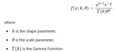
where:
- x is the variable (any positive value).
- k is the shape parameter.
- θ is the scale parameter.
- Γ(k) is the Gamma function, which helps normalize the distribution.
This PDF helps us determine the probability of observing specific values. The shape and scale parameters k and θ influence how the probability density curve looks. When k is small, the curve is steeper and more skewed. As k increases, the curve becomes more spread out.
Key Parameters: Shape (k) and Scale (θ) Explained
The shape parameter k and the scale parameter θ\thetaθ control the look of the Gamma Distribution:
- Shape parameter k: Determines the shape of the curve. When k is low, the distribution is more skewed (leans more to one side). When k is high, it starts to look more like a Normal Distribution.
- Scale parameter θ: Controls how spread out the distribution is. A larger θ stretches the curve, making values less concentrated. Smaller values make the distribution more peaked around lower values.
These parameters together make the Gamma Distribution adaptable to different types of data, from highly skewed to more balanced curves.
Understanding the Mean and Variance of Gamma Distribution
In statistics, the mean and variance help summarize the characteristics of a distribution. For the Gamma Distribution, the mean and variance depend directly on the shape and scale parameters:
- Mean =k×θ: Tells us the average value we can expect. Larger values of k or θ increase the mean.
- Variance =k×θ2: Measures the spread of data around the mean. Larger values of θ\thetaθ create more variability.
How Shape and Scale Affect the Skewness of Gamma Distribution
The skewness, or the degree of asymmetry, in the Gamma Distribution is directly influenced by kkk and θ\thetaθ:
- Higher shape values (k) make the distribution less skewed, gradually creating a more symmetrical, bell-shaped curve.
- Lower shape values create more skew, leaning heavily toward one side, which is useful for representing scenarios where there are many small values but few large ones.
In real-world applications, data scientists and statisticians can adjust k and θ to model different types of skewed data accurately, making the Gamma Distribution versatile for many types of positive-only data.
Must Read
- Why sorted() Is Safer Than list.sort() in Production Python Systems
- Monotonic Sequence in Python: 7 Practical Methods With Edge Cases, Interview Tips, and Performance Analysis
- How to Check if Dictionary Values Are Sorted in Python
- Check If a Tuple Is Sorted in Python — 5 Methods Explained
- How to Check If a List Is Sorted in Python (Without Using sort()) – 5 Efficient Methods
Gamma Function and Its Role in Gamma Distribution
The Gamma Function is a key mathematical concept behind the Gamma Distribution, extending the idea of factorials to non-integer values. In statistics and data science, this function is important for calculating probabilities in the Gamma Distribution, especially for complex shapes and sizes in datasets. It’s often represented as Γ(n) and provides a smooth curve for positive values that helps in various statistical applications.
Let’s dive into what the Gamma Function is, why it’s useful, and how you can implement it in Python to compute the Gamma Distribution.
Definition of Gamma Function in Statistics
The Gamma Function Γ(n) is a generalization of factorials to all positive real numbers. For an integer n, it’s defined as:

This integral-based definition allows the Gamma Function to handle fractional values, which is vital in the Gamma Distribution. In the distribution’s PDF, Γ(k)\Gamma(k)Γ(k) normalizes the probability density function so the total probability sums up to one. This normalization helps ensure that we can use the Gamma Distribution for probability calculations in real-world scenarios.
Calculating Gamma Distribution Using Gamma Function in Python
Let’s go through how to calculate the Gamma Distribution in Python using the SciPy library, which offers convenient functions for the Gamma Function and Gamma Distribution.
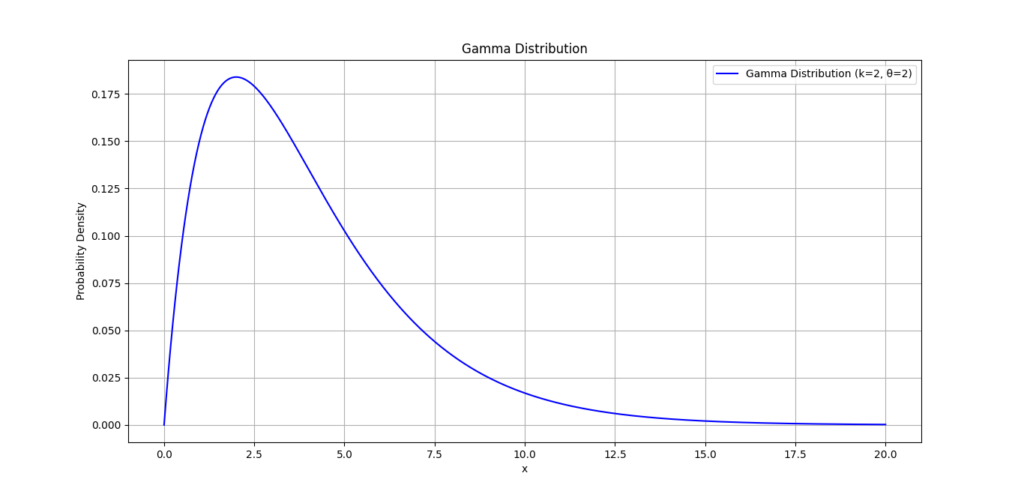
Here’s an example code snippet to calculate and plot the Gamma Distribution in Python:
import numpy as np
import matplotlib.pyplot as plt
from scipy.stats import gamma

# Define the shape (k) and scale (θ) parameters
shape_param = 2  # k
scale_param = 2  # θ

# Generate x values
x = np.linspace(0, 20, 1000)

# Calculate the Gamma Distribution's PDF using the shape and scale parameters
pdf_values = gamma.pdf(x, shape_param, scale=scale_param)

# Plot the distribution
plt.plot(x, pdf_values, label=f'Gamma Distribution (k={shape_param}, θ={scale_param})', color='blue')
plt.xlabel('x')
plt.ylabel('Probability Density')
plt.title('Gamma Distribution')
plt.legend()
plt.grid(True)
plt.show()
Explanation of the Code
- Shape and scale parameters: Here, we define
shape_paramas k=2 andscale_paramas θ=2. You can adjust these values to see how they change the distribution’s shape. - Calculate PDF values: The
gamma.pdf()function from SciPy uses k and θ to calculate the probability density function for the Gamma Distribution. - Plotting: We use Matplotlib to plot the Gamma Distribution’s PDF, helping us visualize how the distribution behaves with our chosen parameters.
Interpreting the Results
The plotted curve shows the probability density of the Gamma Distribution based on the shape and scale values provided. This visual helps us see how likely different values are, which is useful in data analysis for predicting time-to-event data, risk analysis, and other real-world applications.
The Gamma Function allows us to calculate these probabilities accurately, giving the Gamma Distribution the flexibility to model data with skewed or long-tailed distributions effectively. This combination of the Gamma Function and its role in probability calculations makes it essential in fields requiring detailed statistical analysis.
Use Cases of Gamma Distribution in Data Science
Modeling Wait Times and Processes in Queue Theory
In queue theory, the Gamma Distribution is used to model wait times and service processes. When customers arrive at a service point, the time they spend waiting is often not uniform. Instead, it tends to follow a skewed distribution, making the Gamma Distribution a suitable choice.
Mathematical Concept
The Probability Density Function (PDF) of the Gamma Distribution is given by:
Example:
- Imagine a coffee shop during the morning rush. Customers arrive at different times, and each customer takes a varying amount of time to be served.
- The wait times can be modeled using a Gamma Distribution. Here, the shape parameter kkk can represent the number of customers, and the scale parameter θ\thetaθ can reflect the average time spent at the counter.
Python Code Snippet
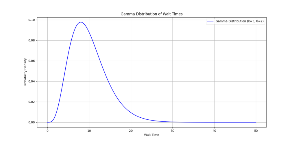
Here’s how you can implement this in Python using the SciPy and Matplotlib libraries:
import numpy as np
import matplotlib.pyplot as plt
from scipy.stats import gamma

# Define the shape (k) and scale (θ) parameters
shape_param = 5  # Example: number of customers
scale_param = 2  # Example: average service time

# Generate x values for the wait times
x = np.linspace(0, 50, 1000)

# Calculate the Gamma Distribution's PDF
pdf_values = gamma.pdf(x, shape_param, scale=scale_param)

# Plot the distribution
plt.plot(x, pdf_values, label=f'Gamma Distribution (k={shape_param}, θ={scale_param})', color='blue')
plt.xlabel('Wait Time')
plt.ylabel('Probability Density')
plt.title('Gamma Distribution of Wait Times')
plt.legend()
plt.grid(True)
plt.show()
This code plots the probability density of wait times, helping businesses understand customer flow.
Risk Analysis and Financial Modeling
In finance, the Gamma Distribution can be instrumental in risk analysis and modeling financial returns. Financial returns often exhibit skewness, which the Gamma Distribution can capture effectively.
Mathematical Concept
The cumulative distribution function (CDF) of the Gamma Distribution helps in determining the probability that a random variable X will take on a value less than or equal to x:

Example:
- Consider an investment portfolio. The returns on investments can be modeled using the Gamma Distribution to evaluate the likelihood of different outcomes.
- Analysts can set the shape and scale parameters to assess potential risks and make informed decisions.
Python Code Snippet
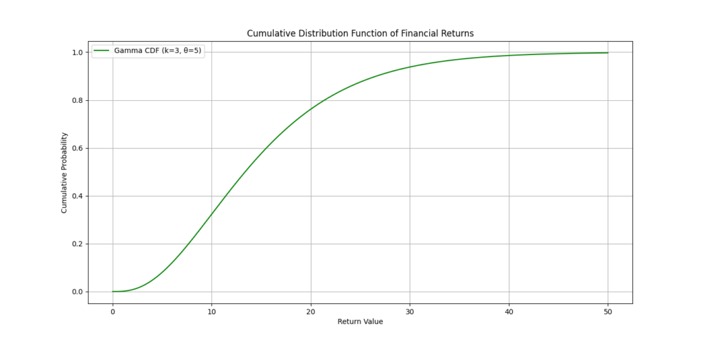
Here’s a Python snippet to visualize the CDF for financial returns:
# Define the parameters for financial modeling
shape_param = 3  # Example: higher for more volatility
scale_param = 5  # Example: average return

# Calculate the CDF of the Gamma Distribution
cdf_values = gamma.cdf(x, shape_param, scale=scale_param)

# Plot the CDF
plt.plot(x, cdf_values, label=f'Gamma CDF (k={shape_param}, θ={scale_param})', color='green')
plt.xlabel('Return Value')
plt.ylabel('Cumulative Probability')
plt.title('Cumulative Distribution Function of Financial Returns')
plt.legend()
plt.grid(True)
plt.show()
This plot helps analysts visualize the likelihood of various return outcomes, enhancing risk assessment.
Reliability and Survival Analysis in Engineering
In engineering, the Gamma Distribution plays a crucial role in reliability and survival analysis. It helps in modeling the time until a failure occurs for mechanical systems or components.
Mathematical Concept
The mean and variance of the Gamma Distribution provide insights into the expected lifespan and variability of components:
Mean=k⋅θ
Variance=k⋅θ2
Example:
- Think of a car engine. Engineers can use the Gamma Distribution to estimate how long the engine is likely to last before needing maintenance or replacement.
Python Code Snippet
Here’s a simple example to calculate the mean and variance:
# Parameters for reliability analysis
shape_param = 4
scale_param = 3

# Calculate mean and variance
mean = shape_param * scale_param
variance = shape_param * (scale_param ** 2)

print(f'Mean lifespan: {mean}')
print(f'Variance: {variance}')
This output helps engineers understand the reliability of components, leading to better design choices.
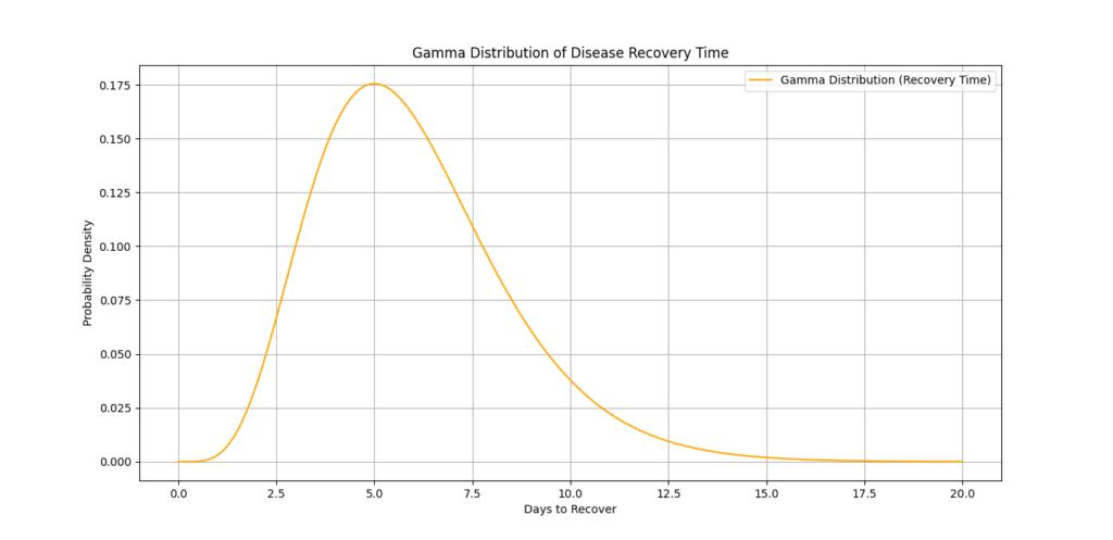
Forecasting in Healthcare (e.g., Modeling Disease Duration)
In healthcare, the Gamma Distribution is useful for modeling the duration of diseases or the time until recovery. It allows healthcare professionals to make predictions based on patient data.
Mathematical Concept
The shape and scale parameters can be adjusted based on historical patient recovery times, allowing for tailored predictions.
Example:
- If a new treatment is introduced for a specific illness, the time taken for patients to recover can be modeled using the Gamma Distribution.
Python Code Snippet
Here’s how you might visualize patient recovery times:
import numpy as np
import matplotlib.pyplot as plt
from scipy.stats import gamma

# Define parameters for healthcare forecasting
shape_param = 6  # Example: reflects more variability in recovery
scale_param = 1  # Example: average days to recover

# Generate x values for recovery times
x_recovery = np.linspace(0, 20, 1000)

# Calculate the PDF for recovery times
pdf_recovery = gamma.pdf(x_recovery, shape_param, scale=scale_param)

# Plot the recovery time distribution
plt.plot(x_recovery, pdf_recovery, label=f'Gamma Distribution (Recovery Time)', color='orange')
plt.xlabel('Days to Recover')
plt.ylabel('Probability Density')
plt.title('Gamma Distribution of Disease Recovery Time')
plt.legend()
plt.grid(True)
plt.show()
This plot can help healthcare providers understand recovery trends and make better resource allocation decisions.
Summary of Use Cases
Here’s a quick overview of the use cases discussed:
| Use Case | Description | Mathematical Concepts |
|---|---|---|
| Queue Theory | Models wait times for customers in service processes, helping optimize staffing and reduce wait times. | PDF and CDF of Gamma Distribution |
| Financial Modeling | Analyzes skewed financial returns for investment portfolios, aiding in risk assessment and decision-making. | CDF and expected outcomes |
| Reliability Analysis | Predicts failure times for engineering components, leading to better design and maintenance strategies. | Mean and variance of the Gamma Distribution |
| Healthcare Forecasting | Models disease duration and recovery times, improving treatment planning and resource allocation. | Parameter adjustments based on historical data |
Why Gamma Distribution is Essential in Bayesian Inference
Bayesian inference is a powerful statistical method that helps us update our understanding of a situation as we gather more data. One of the key ideas in this approach is the prior distribution, which represents our initial beliefs before seeing the data. Among the different types of prior distributions, the Gamma Distribution is particularly useful because of its flexibility and effectiveness.
In this section, we’ll explore why the Gamma Distribution is important in Bayesian inference. We’ll focus on its role as a prior distribution, its use in conjugate priors, and how it’s applied in Bayesian networks and regression models. This will help us see how the Gamma Distribution can improve predictions and insights in various statistical models.
What is a Prior Distribution?
You’re playing a game where you guess how many candies are in a jar. Before you see the jar, you might have some idea, like “I think there are between 10 and 50 candies.” This idea is called a prior distribution. It shows what you believe before you have any evidence.
Why Gamma Distribution?
The Gamma Distribution is a good choice for prior distributions when we are dealing with numbers that can only be positive, like candy counts or the time until something happens (like a light bulb burning out).
Example:
Let’s say you believe a machine will last around 100 hours before it breaks. You can use a Gamma Distribution to represent this belief. If you’re not too sure, you can make it flexible by adjusting its shape.
Using Gamma Distribution as a Conjugate Prior
Now, what happens when you start collecting data? Let’s say you notice the machine breaks at 90 hours, 120 hours, and 110 hours. With Bayesian inference, you can update your belief based on this new information.
What is a Conjugate Prior?
A conjugate prior is a special kind of prior that makes our calculations easier. If we use a Gamma Distribution as a prior for data that follows a Poisson Distribution (like counting events), we can still end up with a Gamma Distribution for our updated belief.
Math Behind It:
- Prior: Think of the prior as your initial belief about something before you have any data. For example, if we believe a machine will last a certain amount of time, we might use a Gamma Distribution to represent that belief.
- Likelihood: The likelihood is about how we interpret new data. In this case, if we observe when the machine breaks, we treat these events as Poisson events, which means they happen randomly but with a known average rate.
- Posterior: After gathering some data (like how often the machine breaks), we update our belief. The updated belief, or posterior, is also represented by a Gamma Distribution, but now it’s adjusted to reflect the new information we have from the observed break times.
Here’s a simple math representation:
- Prior: λ∼Gamma(k,θ)
- Likelihood: X∣λ∼Poisson(λ)
- Posterior: λ∣X∼Gamma(k+sum(X),θ+n)
Practical Applications of Gamma Prior
Now that we know how the Gamma Distribution helps us with our beliefs, let’s look at where we can use it in real life!
1. Modeling Wait Times
Imagine you’re at an amusement park, and you want to know how long people wait for rides. Using a Gamma Distribution can help you predict wait times based on previous data.
2. Risk Analysis in Finance
In finance, we can model risks. If you want to know the chance of losing money in an investment, a Gamma Distribution can help you estimate how likely different outcomes are.
3. Reliability in Engineering
Engineers often want to know how long machines will work before they break down. The Gamma Distribution helps in reliability studies to ensure products are safe and dependable.
4. Healthcare Predictions
In healthcare, we might want to predict how long someone will stay sick. Using a Gamma Distribution allows us to model how long patients take to recover.
Python Example: Using Gamma Distribution
Now, let’s see how we can use the Gamma Distribution in Python! We’ll set up a simple example where we model wait times for a ride at a theme park.
Here’s how you can do it:
import numpy as np
import matplotlib.pyplot as plt
import pymc3 as pm

# Simulating wait times (in minutes)
np.random.seed(42)
wait_times = np.random.gamma(shape=2, scale=3, size=100)  # shape=2, scale=3

# Plotting the simulated wait times
plt.hist(wait_times, bins=30, alpha=0.6, color='b', edgecolor='black')
plt.title('Simulated Wait Times for a Ride')
plt.xlabel('Wait Time (minutes)')
plt.ylabel('Frequency')
plt.show()

# Bayesian model using PyMC3
with pm.Model() as model:
    # Prior distributions for wait time
    alpha = pm.Gamma('alpha', alpha=2, beta=1)
    beta = pm.Gamma('beta', alpha=2, beta=1)

    # Likelihood
    mu = alpha + beta * np.mean(wait_times)  # Mean wait time
    y_obs = pm.Gamma('y_obs', alpha=2, beta=1/mu, observed=wait_times)

    # Sample from the model
    trace = pm.sample(2000, return_inferencedata=False)

# Traceplot of the results
pm.traceplot(trace)
plt.show()
Implementing Gamma Distribution in Python: A Step-by-Step Guide
Setting Up the Python Environment for Gamma Distribution Analysis
Before diving into the code, we need to set up our Python environment. This involves installing and importing some key libraries that will make our analysis easier.
Installing Required Libraries: NumPy, SciPy, and Matplotlib
To start, we need to install the following libraries:
- NumPy: For numerical operations and array manipulation.
- SciPy: To access statistical functions, including those for the Gamma Distribution.
- Matplotlib: For creating visualizations of our data.
To install these libraries, follow these steps:
- Open your terminal or command prompt.
- Run the following commands:
pip install numpy
pip install scipy
pip install matplotlib
Importing and Initializing Libraries for Data Analysis
Once the libraries are installed, we need to import them into our Python script or Jupyter Notebook. Here’s how to do that:
# Importing the necessary libraries
import numpy as np        # For numerical operations
import scipy.stats as stats  # For statistical functions
import matplotlib.pyplot as plt  # For plotting and visualization
With our libraries imported, we’re ready to start generating data and analyzing the Gamma Distribution.
How to Generate Gamma Distribution Data in Python
Now that we have our environment set up, let’s generate some data that follows the Gamma Distribution.
Generating Random Samples Using scipy.stats.gamma.rvs
We can use the scipy.stats.gamma.rvs function to generate random samples from a Gamma Distribution. Here’s how to do it:
# Set parameters for the Gamma Distribution
shape = 2  # Shape parameter (k)
scale = 3  # Scale parameter (θ)
sample_size = 1000  # Number of samples

# Generating random samples
gamma_samples = stats.gamma.rvs(a=shape, scale=scale, size=sample_size)

# Display the first few samples
print(gamma_samples[:10])
Creating Custom Gamma Distribution with Varying Parameters
You can easily create custom Gamma Distributions by varying the shape and scale parameters. For example:
# Different parameters for Gamma Distribution
shape_1 = 2
scale_1 = 1

shape_2 = 5
scale_2 = 2

# Generate samples for both distributions
samples_1 = stats.gamma.rvs(a=shape_1, scale=scale_1, size=sample_size)
samples_2 = stats.gamma.rvs(a=shape_2, scale=scale_2, size=sample_size)

# Print the first few samples
print("Samples from Distribution 1:", samples_1[:10])
print("Samples from Distribution 2:", samples_2[:10])
Visualizing Gamma Distribution Data with Matplotlib
Now that we have our samples, let’s visualize them using Matplotlib. A histogram can help us understand the shape of our Gamma Distribution:
# Plotting the histogram of the samples
plt.figure(figsize=(10, 6))
plt.hist(gamma_samples, bins=30, alpha=0.6, color='blue', edgecolor='black')
plt.title('Histogram of Random Samples from Gamma Distribution')
plt.xlabel('Value')
plt.ylabel('Frequency')
plt.grid(True)
plt.show()
Fitting Data to Gamma Distribution
After generating data, we can fit it to the Gamma Distribution using statistical methods. This involves finding the best-fitting parameters for our data.
Using Maximum Likelihood Estimation (MLE) to Fit Gamma Distribution
Maximum Likelihood Estimation (MLE) is a common method for estimating parameters in statistical models. Here’s how to fit our data using MLE:
# Fit the data to a Gamma Distribution
params = stats.gamma.fit(gamma_samples)

# Extract the parameters
shape_fit, loc_fit, scale_fit = params
print(f'Fitted Parameters: Shape = {shape_fit}, Location = {loc_fit}, Scale = {scale_fit}')
Measuring Goodness-of-Fit for Gamma Distribution Models
To evaluate how well our Gamma Distribution fits the data, we can use methods like the Kolmogorov-Smirnov test. This test compares our sample data to the theoretical distribution.
# Performing the Kolmogorov-Smirnov test
D, p_value = stats.kstest(gamma_samples, 'gamma', args=params)
print(f'K-S Statistic: {D}, p-value: {p_value}')
A high p-value (above 0.05) suggests that the fit is acceptable.
Practical Example: Fitting Gamma Distribution to a Real Dataset
Let’s put this all together by fitting a Gamma Distribution to a real dataset. You can use any dataset that contains positive continuous values. For this example, let’s assume we have a dataset of wait times at a service center.
# Example dataset of wait times (in minutes)
wait_times = [2.5, 3.0, 2.2, 4.5, 1.5, 3.6, 2.9, 4.0, 3.3, 2.7]

# Fit the wait times to a Gamma Distribution
params_wait_times = stats.gamma.fit(wait_times)

# Print the fitted parameters
print(f'Fitted Parameters for Wait Times: Shape = {params_wait_times[0]}, Location = {params_wait_times[1]}, Scale = {params_wait_times[2]}')
Example 1: Modeling Customer Wait Time with Gamma Distribution
In this example, we’ll explore how to model customer wait times using the Gamma Distribution. This approach helps businesses understand customer experiences better, leading to improved service and satisfaction. Let’s break this down step by step.
Scenario and Data Preparation
Imagine you own a coffee shop. During busy hours, customers often wait a bit longer for their orders. You want to figure out how long they typically wait so you can adjust staffing levels and improve the overall experience.
Data Collection
Let’s say you collected wait times (in minutes) for 20 customers during peak hours:
- Wait Times: [1.5, 2.3, 3.0, 2.5, 1.8, 2.1, 2.7, 3.2, 3.5, 4.0, 2.0, 1.9, 2.4, 3.1, 2.6, 4.2, 3.8, 2.8, 3.6, 4.5]
This data will help us fit a Gamma Distribution to analyze customer wait times effectively.
Python Code for Modeling Wait Times
Now, let’s write some Python code to model the customer wait times using the Gamma Distribution. We’ll use a few libraries to make our analysis easier.
Step 1: Importing Libraries
First, we need to import the necessary libraries for our analysis.
# Importing necessary libraries
import numpy as np
import scipy.stats as stats
import matplotlib.pyplot as plt
Step 2: Data Preparation
Next, we’ll prepare our wait times data as a NumPy array.
# Defining wait times data
wait_times = np.array([1.5, 2.3, 3.0, 2.5, 1.8, 2.1, 2.7, 3.2, 3.5, 4.0,
2.0, 1.9, 2.4, 3.1, 2.6, 4.2, 3.8, 2.8, 3.6, 4.5])
Step 3: Fitting the Gamma Distribution
Now, we will fit the Gamma Distribution to our wait times using Maximum Likelihood Estimation (MLE).
# Fitting the Gamma Distribution to the wait times
shape, loc, scale = stats.gamma.fit(wait_times)
# Displaying the fitted parameters
print(f'Fitted Parameters:\nShape (k) = {shape:.2f}\nLocation (loc) = {loc:.2f}\nScale (θ) = {scale:.2f}')
Step 4: Generating Data Points for the Gamma Distribution Curve
Next, we need to generate data points to visualize our fitted Gamma Distribution.
# Generating x values for the curve
x = np.linspace(0, 5, 100)
# Calculating the corresponding y values for the Gamma Distribution
y = stats.gamma.pdf(x, a=shape, loc=loc, scale=scale)
Step 5: Plotting the Results
Finally, we’ll visualize the original wait times and the fitted Gamma Distribution.
# Plotting the wait times and the Gamma Distribution
plt.figure(figsize=(10, 6))
plt.hist(wait_times, bins=10, density=True, alpha=0.5, color='blue', label='Wait Times (Histogram)')
plt.plot(x, y, 'r-', lw=2, label='Fitted Gamma Distribution')
plt.title('Customer Wait Times and Fitted Gamma Distribution')
plt.xlabel('Wait Time (minutes)')
plt.ylabel('Density')
plt.legend()
plt.grid()
plt.show()
Output :
Fitted Parameters:
Shape (k) = 5.75
Location (loc) = 0.81
Scale (θ) = 0.36
Analyzing Results and Interpreting the Gamma Distribution Curve
After running the code, you will see a histogram of customer wait times alongside the fitted Gamma Distribution curve.
Interpreting the Results
- Shape of the Curve: The curve’s shape reveals the likelihood of different wait times. A peak at a specific time indicates that most customers wait around that value.
- Fitted Parameters:
- Shape (k): This parameter shows how the data is skewed. A shape less than 1 suggests left-skewed data, while a shape greater than 1 indicates right-skewed data.
- Scale (θ): A larger scale value indicates longer wait times.
- Understanding Density: The y-axis represents probability density. A higher density means a greater likelihood of that wait time occurring.
Example 2: Using Gamma Distribution in Reliability Analysis
In this example, we will look at how the Gamma Distribution can be used in reliability analysis. Understanding how long a product lasts before it fails is crucial for businesses. It helps improve designs, enhance customer satisfaction, and manage warranties effectively. Let’s break it down step by step.
Introduction to Reliability Analysis
Reliability analysis focuses on the ability of a product or system to perform its intended function without failure over a specified period. Businesses need to know when products are likely to fail to improve designs, reduce costs, and enhance customer satisfaction.
Why Use Gamma Distribution?
The Gamma Distribution is especially useful in reliability analysis for several reasons:
- Flexible Shape: It can model various failure rates, making it suitable for different types of products.
- Positive Values: It only takes positive values, aligning with real-world situations where failure times can’t be negative.
- Skewness: It can accommodate skewed data, which is common in real-world scenarios where some products fail much sooner than others.
Python Code for Gamma Distribution in Reliability Analysis
Now, let’s write some Python code to analyze product reliability using the Gamma Distribution. We will simulate failure times of a product.
Step 1: Importing Libraries
First, we need to import the necessary libraries.
# Importing necessary libraries
import numpy as np
import scipy.stats as stats
import matplotlib.pyplot as plt
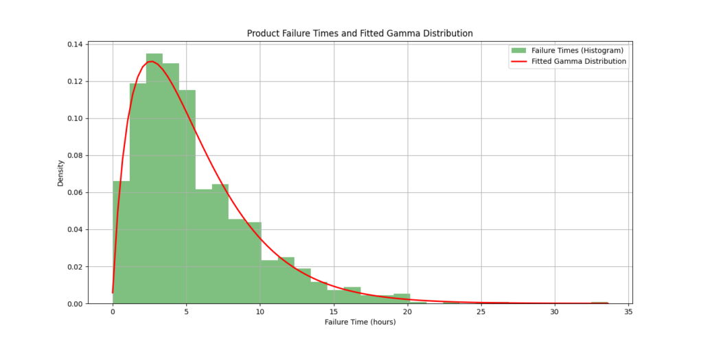
Step 2: Simulating Failure Times
We will simulate failure times for a product based on a Gamma Distribution. Let’s say we want to analyze the lifetime of a certain electronic device.
# Simulating failure times using Gamma Distribution
shape = 2.0   # Shape parameter (k)
scale = 3.0   # Scale parameter (θ)
size = 1000   # Number of simulated failure times

# Generating failure times
failure_times = np.random.gamma(shape, scale, size)
Step 3: Fitting the Gamma Distribution
Now, we will fit the simulated failure times to a Gamma Distribution using Maximum Likelihood Estimation (MLE).
# Fitting the Gamma Distribution to the simulated failure times
fitted_shape, loc, fitted_scale = stats.gamma.fit(failure_times)

# Displaying the fitted parameters
print(f'Fitted Parameters:\nShape (k) = {fitted_shape:.2f}\nLocation (loc) = {loc:.2f}\nScale (θ) = {fitted_scale:.2f}')
Step 4: Visualizing Reliability and Failure Rates
Next, we will visualize the failure times and the fitted Gamma Distribution.
# Generating x values for the curve
x = np.linspace(0, max(failure_times), 100)

# Calculating the corresponding y values for the Gamma Distribution
y = stats.gamma.pdf(x, a=fitted_shape, loc=loc, scale=fitted_scale)

# Plotting the failure times and the fitted Gamma Distribution
plt.figure(figsize=(10, 6))
plt.hist(failure_times, bins=30, density=True, alpha=0.5, color='green', label='Failure Times (Histogram)')
plt.plot(x, y, 'r-', lw=2, label='Fitted Gamma Distribution')
plt.title('Product Failure Times and Fitted Gamma Distribution')
plt.xlabel('Failure Time (hours)')
plt.ylabel('Density')
plt.legend()
plt.grid()
plt.show()
Output:
Fitted Parameters:
Shape (k) = 1.89
Location (loc) = -0.03
Scale (θ) = 2.96
Interpreting the Results
- Shape of the Curve: The curve illustrates how often different failure times occur. A peak at a certain time indicates that many products are likely to fail around that time.
- Fitted Parameters:
- Shape (k): This indicates the distribution of failure times. A higher shape value suggests more consistency in failure times, while a lower value indicates greater variability.
- Scale (θ): A larger scale value shows that, on average, the products last longer before failing.
- Understanding Density: The y-axis represents the probability density of failure times. A higher density indicates that the product is more likely to fail around that time.
Latest Advancements in Gamma Distribution for Data Science
The Gamma Distribution has been a significant tool in statistics and data science. Recently, its applications have expanded with advancements in technology and analytics. Let’s explore the latest trends in using the Gamma Distribution within various fields of data science.
AI-Powered Gamma Distribution Estimation in Large Datasets
In today’s world, the size of datasets has exploded, making it increasingly challenging to perform statistical analyses. However, advancements in artificial intelligence (AI) have transformed how we estimate Gamma Distribution parameters.
Automated Estimation Techniques
- Machine Learning Algorithms: Algorithms like gradient boosting and neural networks are now being used to estimate parameters for the Gamma Distribution in large datasets. These models can automatically identify patterns and optimize parameter estimates.
- Parallel Processing: Techniques such as parallel computing allow for quicker processing of large datasets, enabling real-time updates to the estimated distribution parameters. This is particularly useful in industries like finance and healthcare, where decisions need to be made rapidly.
Example
Imagine you are analyzing customer purchase times in an e-commerce platform. AI algorithms can learn from historical purchase data, estimating the Gamma Distribution parameters that represent wait times. This analysis can help in predicting future purchase behavior, optimizing inventory levels, and enhancing customer experience.
Using Gamma Distribution for Time Series Forecasting
Time series forecasting is crucial in various sectors, including finance, retail, and meteorology. The Gamma Distribution plays an essential role in modeling events that occur over time.
Key Features
- Handling Skewed Data: Many time series datasets exhibit skewness. The Gamma Distribution can effectively model this skewness, providing more accurate predictions.
- Dynamic Modeling: With the Gamma Distribution, you can model changes over time, which is especially useful for understanding trends and seasonality in data.
Practical Application
Consider predicting daily sales for a retail store. By applying the Gamma Distribution to historical sales data, you can forecast future sales trends, helping to manage stock levels and promotions.
Applications of Gamma Distribution in Deep Learning and Neural Networks
Deep learning has revolutionized data science, and the Gamma Distribution has found its place in this advanced landscape.
Key Areas of Use
- Activation Functions: Some neural network architectures utilize Gamma Distribution as an activation function. This can enhance model performance, especially in tasks involving regression.
- Loss Functions: The Gamma Distribution can also be used in defining loss functions for models predicting positive continuous outcomes, providing better optimization for certain datasets.
Example
In a neural network designed to predict insurance claims, using a Gamma Distribution as a loss function can improve accuracy. This is because insurance claims are often non-negative and can be heavily skewed, making the Gamma Distribution an ideal fit.
Using Gamma Distribution in Reinforcement Learning and Decision-Making Models
Reinforcement learning (RL) is about making optimal decisions based on the rewards received from previous actions. The Gamma Distribution can enhance decision-making models in RL.
Benefits of Gamma Distribution in RL
- Modeling Uncertainty: The Gamma Distribution can effectively model the uncertainty of rewards in RL scenarios, providing a more nuanced approach to decision-making.
- Continuous Action Spaces: In problems where the actions have continuous outcomes, such as robotics and finance, the Gamma Distribution can be used to model the probabilities of different outcomes, guiding the agent’s learning process.
Real-World Example
Imagine a robot learning to navigate a maze. By using the Gamma Distribution to model the uncertainties associated with each path, the robot can make informed decisions about which direction to take, improving its chances of finding the exit efficiently.
Visualizing Gamma Distribution: Tips for Better Insights
Visualizing the Gamma Distribution is essential for understanding its properties and making data-driven decisions. Effective visualizations can help reveal trends, patterns, and relationships in your data. In this section, we’ll explore different visualization techniques, including heatmaps, histograms, and density plots, while also diving into how to create interactive visualizations with Python. We’ll also compare the Gamma Distribution with exponential and normal distributions graphically.
Heatmaps, Histograms, and Density Plots for Gamma Distribution
Visualizations like heatmaps, histograms, and density plots can provide valuable insights into the Gamma Distribution.
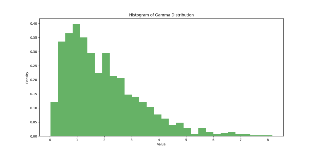
Histograms
- Purpose: A histogram displays the distribution of your data by showing the frequency of data points within specified intervals (bins).
- Creating a Histogram: You can create a histogram using Matplotlib, which provides a clear view of how your data is distributed.
Example: Creating a Histogram for Gamma Distribution
import numpy as np
import matplotlib.pyplot as plt
from scipy.stats import gamma

# Parameters for the Gamma Distribution
shape = 2  # Shape parameter (k)
scale = 1  # Scale parameter (θ)

# Generate random samples
data = gamma.rvs(shape, scale=scale, size=1000)

# Create histogram
plt.hist(data, bins=30, density=True, alpha=0.6, color='g')

# Add title and labels
plt.title('Histogram of Gamma Distribution')
plt.xlabel('Value')
plt.ylabel('Density')

# Show the plot
plt.show()
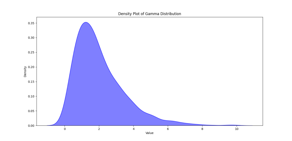
Density Plots
- Purpose: Density plots provide a smooth estimate of the distribution’s probability density function (PDF). This is useful for visualizing the shape of the distribution.
- Creating a Density Plot: You can use Seaborn, a Python library built on Matplotlib, to easily create density plots.
Example: Creating a Density Plot for Gamma Distribution
import numpy as np
import matplotlib.pyplot as plt
import seaborn as sns
from scipy.stats import gamma

# Parameters for the Gamma Distribution
shape = 2  # Shape parameter (k)
scale = 1  # Scale parameter (θ)

# Generate random samples
data = gamma.rvs(shape, scale=scale, size=1000)

# Create density plot
sns.kdeplot(data, fill=True, color='blue', alpha=0.5)

# Add title and labels
plt.title('Density Plot of Gamma Distribution')
plt.xlabel('Value')
plt.ylabel('Density')

# Show the plot
plt.show()
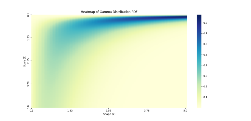
Heatmaps
- Purpose: Heatmaps are useful for visualizing the relationship between two variables. They can help you understand how different parameters affect the Gamma Distribution.
- Creating a Heatmap: You can use
numpyandseabornto create heatmaps for two-dimensional data.
Example: Creating a Heatmap for Gamma Distribution Parameters
# Create a grid of shape and scale values
shape_values = np.linspace(0.1, 5, 100)
scale_values = np.linspace(0.1, 5, 100)
X, Y = np.meshgrid(shape_values, scale_values)

# Calculate the Gamma PDF for each combination of shape and scale
Z = gamma.pdf(1, a=X, scale=Y)

# Create heatmap
plt.figure(figsize=(10, 6))
sns.heatmap(Z, extent=(0.1, 5, 0.1, 5), origin='lower', cmap='YlGnBu')
plt.title('Heatmap of Gamma Distribution PDF')
plt.xlabel('Shape (k)')
plt.ylabel('Scale (θ)')

# Show the plot
plt.show()
Creating Interactive Visualizations with Python Plotting Libraries
Interactive visualizations can enhance your understanding of the Gamma Distribution by allowing you to explore the data dynamically. Libraries like Plotly and Bokeh can help you create interactive plots.
Example: Using Plotly for Interactive Plots
import plotly.express as px

# Create a DataFrame for the Gamma Distribution data
df = pd.DataFrame({'Data': data})

# Create an interactive histogram
fig = px.histogram(df, x='Data', title='Interactive Histogram of Gamma Distribution', nbins=30)
fig.update_traces(opacity=0.75)
fig.show()
With Plotly, you can hover over the bars to see the exact values, zoom in on areas of interest, and toggle different views.
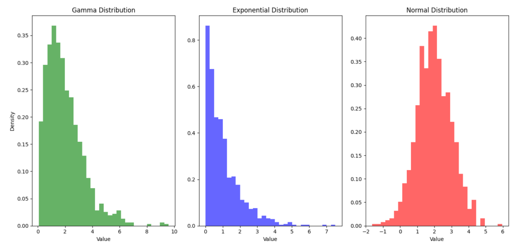
Comparing Gamma Distribution with Exponential and Normal Distributions Graphically
Visual comparisons between the Gamma Distribution, exponential distribution, and normal distribution can highlight their differences.
Example: Comparative Visualization
# Generate random samples for Gamma, Exponential, and Normal distributions
import numpy as np
from matplotlib import pyplot as plt
from scipy.stats import gamma

# Generate Gamma distribution data
shape = 2  # Shape parameter for Gamma
scale = 1  # Scale parameter for Gamma
data = gamma.rvs(shape, scale=scale, size=1000)

# Generate Exponential and Normal distribution data
exp_data = np.random.exponential(scale=1, size=1000)
norm_data = np.random.normal(loc=2, scale=1, size=1000)

# Create a figure for comparison
plt.figure(figsize=(12, 6))

# Histogram for Gamma Distribution
plt.subplot(1, 3, 1)
plt.hist(data, bins=30, density=True, alpha=0.6, color='g')
plt.title('Gamma Distribution')
plt.xlabel('Value')
plt.ylabel('Density')

# Histogram for Exponential Distribution
plt.subplot(1, 3, 2)
plt.hist(exp_data, bins=30, density=True, alpha=0.6, color='b')
plt.title('Exponential Distribution')
plt.xlabel('Value')

# Histogram for Normal Distribution
plt.subplot(1, 3, 3)
plt.hist(norm_data, bins=30, density=True, alpha=0.6, color='r')
plt.title('Normal Distribution')
plt.xlabel('Value')

# Show the plots
plt.tight_layout()
plt.show()
Insights from the Comparison
- Shape Differences: The Gamma Distribution can be skewed, while the exponential distribution is memoryless, and the normal distribution is symmetric.
- Applications: Understanding these differences helps in selecting the appropriate distribution based on the nature of your data.
Interpreting Gamma Distribution Graphs for Better Decision-Making
Understanding the Gamma Distribution is crucial for making informed decisions in data science. The way we visualize this distribution can reveal important patterns and insights about our data. In this section, we will explore how to interpret Gamma Distribution graphs effectively, how to use these plots to drive data science decisions, and common misinterpretations to watch out for.
Understanding Shape and Scale Variations Through Graphs
The Gamma Distribution is characterized by two key parameters: shape (k) and scale (θ). These parameters significantly influence the appearance of the distribution graph.
Shape Parameter (k)
- Definition: The shape parameter determines the form of the distribution.
- Effects:
- When k < 1, the distribution is highly skewed to the right.
- When k = 1, it behaves like an exponential distribution.
- When k > 1, the distribution becomes more symmetric and bell-shaped.
Scale Parameter (θ)
- Definition: The scale parameter stretches or compresses the distribution along the x-axis.
- Effects:
- A larger θ results in a wider spread of values.
- A smaller θ makes the distribution more concentrated around the mean.
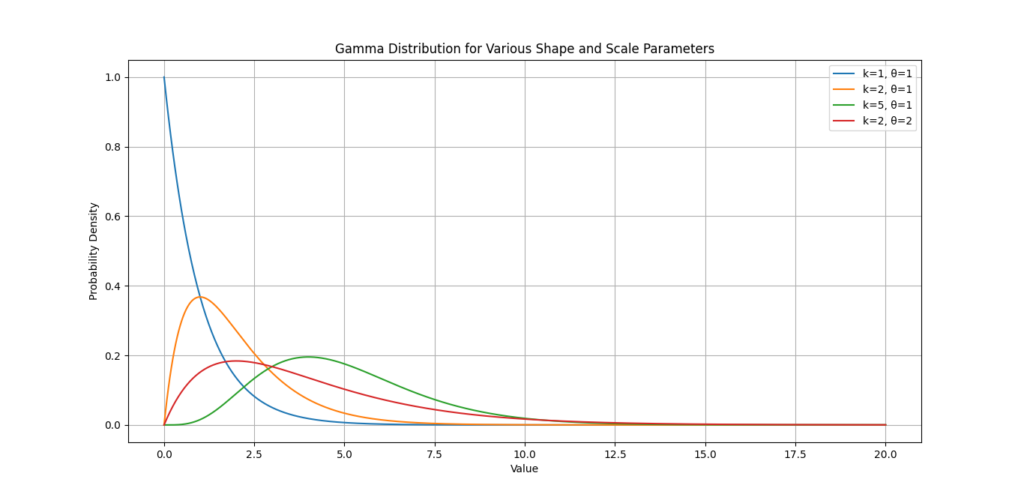
Example: Visualizing the Effects of Shape and Scale
Here’s how changing the shape and scale parameters impacts the Gamma Distribution:
import numpy as np
import matplotlib.pyplot as plt
from scipy.stats import gamma

# Define different parameters
params = [(1, 1), (2, 1), (5, 1), (2, 2)]

# Create plots
plt.figure(figsize=(12, 8))
x = np.linspace(0, 20, 1000)

for shape, scale in params:
    plt.plot(x, gamma.pdf(x, a=shape, scale=scale), label=f'k={shape}, θ={scale}')

plt.title('Gamma Distribution for Various Shape and Scale Parameters')
plt.xlabel('Value')
plt.ylabel('Probability Density')
plt.legend()
plt.grid()
plt.show()
Insights from the Graph
- By observing the variations in shape and scale, you can assess how likely certain outcomes are. For example, if you see a distribution skewed to the right, it might suggest that higher wait times are more likely, helping businesses prepare accordingly.
Using Gamma Distribution Plots to Inform Data Science Decisions
Gamma distribution plots are not just for analysis; they can also inform strategic decisions in various fields, including healthcare, finance, and engineering.
Applications in Decision-Making
- Risk Assessment: By modeling wait times or failure rates, organizations can better manage risks and plan for unexpected delays.
- Resource Allocation: Understanding the distribution of outcomes can guide resource allocation more effectively, ensuring that critical areas are adequately staffed or supplied.
- Predictive Analysis: Data scientists can use the Gamma Distribution to forecast future events based on historical data, improving decision-making processes.
Example: Analyzing Customer Wait Times
Imagine a restaurant analyzing customer wait times to improve service:
- Data Collection: Gather historical data on customer wait times.
- Gamma Distribution Modeling: Fit a Gamma Distribution to this data.
- Decision Implementation: Use insights from the distribution to adjust staffing during peak hours.
Common Misinterpretations and How to Avoid Them
While interpreting Gamma Distribution graphs, several common misinterpretations can lead to poor decision-making. Here’s how to avoid them:
Misinterpretation 1: Confusing Shape with Central Tendency
- Issue: A skewed distribution may lead to an overemphasis on the mean, which could be misleading.
- Solution: Focus on the median or mode when discussing central tendency in skewed distributions.
Misinterpretation 2: Ignoring Parameter Influence
- Issue: Not recognizing how shape and scale parameters interact can lead to incorrect conclusions about variability and risk.
- Solution: Always examine the parameters in your analysis and understand their implications on the distribution.
Misinterpretation 3: Overgeneralizing Findings
- Issue: Drawing broad conclusions based on a limited dataset can lead to faulty predictions.
- Solution: Ensure a sufficient sample size and consider the context before making conclusions.
Example: Avoiding Misinterpretations in Decision-Making
Let’s say you analyze a Gamma Distribution for a product failure rate and find that the mean failure time is 10 hours. If the distribution is highly skewed, assuming that the product will fail around the 10-hour mark could be misleading. Instead, consider the variance and the shape of the distribution to understand the risk more comprehensively.
Conclusion: Using Gamma Distribution in Data Science
In this blog post, we explored Gamma Distribution in Data Science and why it is important. This tool helps us understand and model many real-world situations. For example, we can use it to analyze customer wait times or assess risks in finance.
We learned about the key parts of the Gamma Distribution, like shape and scale. These parameters help us customize our analyses to fit specific needs. We also saw how to apply this knowledge using Python. By using libraries like NumPy, SciPy, and Matplotlib, we can easily generate random samples, visualize data, and fit models to real datasets.
The Gamma Distribution is useful in many areas. It goes beyond traditional applications. For instance, we can use it in AI to estimate data and in forecasting future trends. These advancements show how powerful the Gamma Distribution can be for data analysis.
By adding the Gamma Distribution to your skills, you can make better decisions and understand data more deeply. Whether you are experienced or just starting, this distribution can help you analyze data effectively.
In short, the Gamma Distribution is a helpful tool in data science. It allows us to gain insights and make smarter choices. As you use what you’ve learned, keep exploring and practicing. The world of data science has many opportunities waiting for you!
External Resources
Towards Data Science: “Understanding the Gamma Distribution”
- This blog post provides an accessible explanation of the Gamma distribution, its properties, and applications in data science.
- Understanding the Gamma Distribution
NumPy Documentation
- The NumPy documentation provides guidance on statistical functions and random number generation, including the Gamma distribution.
- NumPy Documentation
Matplotlib Documentation
- Matplotlib documentation explains how to visualize data, including how to create plots for distributions like the Gamma distribution.
- Matplotlib Documentation
FAQs
1. What is Gamma Distribution?
The Gamma distribution is a continuous probability distribution commonly used to model wait times, failure rates, and other data that are always positive. It is defined by two parameters: shape (k) and scale (θ).
2. When should I use Gamma Distribution instead of other distributions?
Use the Gamma distribution when modeling data that is skewed and strictly positive, such as wait times or service times. It is often preferred over the normal distribution when the data does not fit a symmetric pattern.
3. How can I visualize Gamma Distribution in Python?
You can visualize the Gamma distribution using libraries like Matplotlib and SciPy. By generating random samples with scipy.stats.gamma.rvs and plotting them with Matplotlib, you can create histograms and density plots to illustrate the distribution’s shape.
4. What are the practical applications of Gamma Distribution in data science?
The Gamma distribution is used in various applications, such as modeling customer wait times, reliability analysis in engineering, risk assessment in finance, and forecasting in healthcare. It helps data scientists make informed decisions based on the behavior of real-world phenomena.






Leave a Reply