Probability Distribution in Data Science
Introduction: Probability Distribution in Data Science
Have you ever noticed that certain things seem to happen more often than others? Like, you might see sunny days more often than snowy ones, or get more A’s and B’s than F’s on your report card. Probability distribution is a way to show where things tend to happen the most and where they don’t.
Think of it like this: imagine we counted how many times each grade showed up on your report card. A probability distribution would help us see which grades you got most often and which ones were rare. This idea is super useful in data science because it helps us understand all kinds of patterns in data.
In this blog, we’ll explore how probability distributions work. We’ll look at different types, like the normal distribution (which often looks like a hill) and others with different shapes. By the end, you’ll see how knowing about probability makes it easier to predict things and make smarter choices with data.
Let’s get started and discover the world of probability together!
What Are Probability Distributions in Data Science?
In data science, probability distributions are like roadmaps that tell us where data points are likely to appear. They help us predict what values are common, which ones are rare, and give us insight into the data’s overall shape. Probability distributions make it easier for data scientists and machine learning models to understand the patterns within data and predict future outcomes.
Why Probability Distributions Are Important in Data Science
Probability distributions help people make smart guesses based on patterns they see in data. Here’s why they’re so useful in data science and machine learning:
Training Machines to Recognize Patterns
Probability distributions also help machines learn. When we give machines data that follows certain patterns, it’s easier for them to recognize those patterns in new data.
Understanding Patterns
Probability distributions help people see patterns in data. For example, if you’re counting how many times people buy ice cream each day, a probability distribution can help show that ice cream sales are high in summer and lower in winter.
Predicting What Will Happen
With probability distributions, data scientists can make predictions. For example:
In a school, they can predict how many students might score A’s or B’s on a test.
In a store, they can predict how many people will visit on a busy day.
How Probability Distributions Help Us Make Decisions
Probability distributions help people make better choices by giving clues about what’s likely to happen. Here’s how they do it:
- Avoiding Surprises: By studying probability distributions, we can guess what might happen next. For example, if a zoo sees that most visitors come on weekends, they know to prepare for big crowds on those days.
- Planning Resources: Businesses use probability distributions to figure out what they need and when. For example, a pizza shop might use it to plan how much pizza dough to make on a Friday night compared to a Monday afternoon.
Types of Probability Distributions in Data Science
Overview of Key Probability Distribution Types
Probability distributions can be divided into two main groups: Discrete and Continuous. Each type serves different purposes and comes with unique characteristics:
- Discrete Probability Distributions: These are used when the outcomes are countable or have specific, separate values. For instance, if you’re counting the number of students in a class, that’s discrete since you can’t have half a student. Examples include the Binomial and Poisson distributions.
- Continuous Probability Distributions: These are used when the data can take any value within a given range. Heights of students or the time it takes to finish a test would be examples of continuous data. Examples of continuous distributions include the Normal and Exponential distributions.
Categorizing Probability Distributions: Discrete vs. Continuous
Here’s a breakdown of these categories and some of the most common types within each:
1. Discrete Probability Distributions
Discrete distributions apply when outcomes can only take specific values. This category is perfect for data like counts or yes/no outcomes.
- Binomial Distribution
- Purpose: Predicts outcomes with two possibilities, like success/failure.
- Example: The number of heads when flipping a coin multiple times.
- Where It’s Used: Often in A/B testing and decision-making situations.
- Poisson Distribution
- Purpose: Shows the number of events that happen in a fixed period or area.
- Example: Counting the number of people arriving at a store in an hour.
- Where It’s Used: Useful in customer service to predict call volumes or event rates.
2. Continuous Probability Distributions
Continuous distributions apply when data can take any value in a range, like height, weight, or temperature. These distributions help with measurements that can vary continuously.
- Normal Distribution (Bell Curve)
- Purpose: This is the classic bell curve, where most data points are near the mean, and fewer points fall toward the edges.
- Example: Heights of students in a class, where most heights are around the average.
- Where It’s Used: Frequently used in grading and forecasting since it’s predictable and common.
- Exponential Distribution
- Purpose: Used for data that shows time until an event happens, like the time before a light bulb burns out.
- Example: Predicting the lifespan of electronic devices.
- Where It’s Used: Commonly applied in reliability testing and queuing theory.
Quick Comparison of Discrete and Continuous Distributions
| Distribution Type | Discrete or Continuous | Example | Common Use Cases |
|---|---|---|---|
| Binomial | Discrete | Flipping a coin (Heads or Tails) | A/B testing, surveys |
| Poisson | Discrete | Count of arrivals at a store | Customer service, events |
| Normal | Continuous | Heights of individuals | Grading, forecasting |
| Exponential | Continuous | Time until a light bulb burns out | Reliability, queuing |
Why Learn About Different Probability Distributions?
Each distribution type helps data scientists and analysts understand, analyze, and interpret different data patterns. Knowing which type of probability distribution to use allows data science professionals to:
- Choose the Right Analysis: Using the right probability distribution leads to more accurate predictions.
- Make Better Predictions: By understanding distribution types, it’s easier to forecast outcomes like customer behavior or product lifespans.
- Solve Real-Life Problems: Distributions are used in everything from planning store inventory to predicting election results.
When data scientists have a solid understanding of probability distribution types, they can make more confident and accurate decisions based on data.
Discrete Probability Distributions
A discrete probability distribution is a way to show the chances of different outcomes that can only be whole numbers. For example:
- If you roll a die, you can get 1, 2, 3, 4, 5, or 6. These are specific numbers you can count, and they don’t include anything in between (like 2.5).
- When we add up the chances of all possible outcomes, we always get 1 (or 100%). This means something must happen every time.
Here are some important points about discrete probability distributions:
- Countable Outcomes: You can list all possible outcomes, like the number of pets you have (0, 1, 2, 3…).
- Fixed Total: If you add all the probabilities (the chances of each outcome), they will equal 1.
Common types of discrete probability distributions include the Binomial, Poisson, and Geometric distributions.
Real-Life Applications of Discrete Distributions in Data Science
Now, let’s look at how discrete probability distributions are used in real life:
- Binomial Distribution
- What It Is: This distribution is used when you have two options, like yes/no or success/failure.
- Example: Think about a quiz where you guess on 10 questions. The binomial distribution can help you figure out how many questions you might get right.
- How It’s Used: Companies use this to test things, like deciding which advertisement works better by counting the number of people who liked each ad.
- Poisson Distribution
- What It Is: This distribution helps us predict how many times something will happen in a certain time frame.
- Example: Imagine you’re counting how many people come into a store every hour. The Poisson distribution can tell you how many customers to expect.
- How It’s Used: Businesses use this to prepare for busy times, like having enough staff during sales or holidays.
- Geometric Distribution
- What It Is: This distribution is about how long it takes to get the first success.
- Example: If you flip a coin, the geometric distribution can help you figure out how many times you’ll flip it before you get heads.
- How It’s Used: It’s helpful for testing products, like figuring out how many tries it takes to find a defective toy on a production line.
Quick Comparison of Discrete Probability Distributions
| Distribution Type | What It Measures | Example | How It’s Used |
|---|---|---|---|
| Binomial | Two outcomes (like yes or no) | Number of questions answered correctly | Testing ads, surveys |
| Poisson | Number of events in a time period | Customers coming into a store in an hour | Planning for busy times |
| Geometric | Number of tries until first success | Flips to get heads on a coin | Quality testing, production checks |
Binomial Distribution: Understanding with Math and Python
The binomial distribution is a key concept in probability and statistics, especially useful in data science when we deal with two-outcome events, like success/failure, true/false, or yes/no situations. It’s widely applied in A/B testing and classification tasks in machine learning to help predict and validate results.
Mathematical Formula of the Binomial Distribution
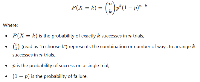
The binomial distribution formula calculates the probability of obtaining exactly kkk successes in nnn trials, where each trial has a probability ppp of success.
The formula is:
Let’s calculate this in Python.
Binomial Distribution in Python
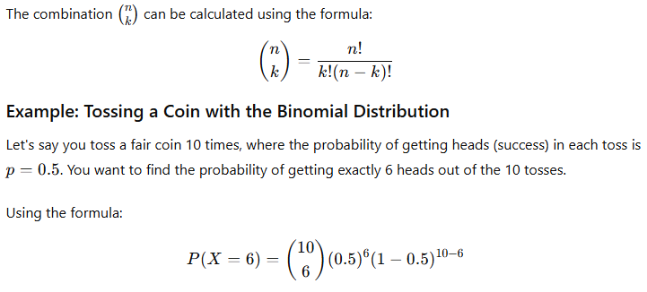
Python’s scipy.stats library provides a simple way to calculate binomial probabilities. Let’s use it to find the probability of getting exactly 6 heads out of 10 tosses.
from scipy.stats import binom

# Parameters
n = 10      # Number of trials (tosses)
k = 6       # Desired number of successes (heads)
p = 0.5     # Probability of success on each trial (probability of heads)

# Calculate binomial probability
probability = binom.pmf(k, n, p)
print(f"The probability of getting exactly {k} heads out of {n} tosses is: {probability:.4f}")
Visualizing the Binomial Distribution
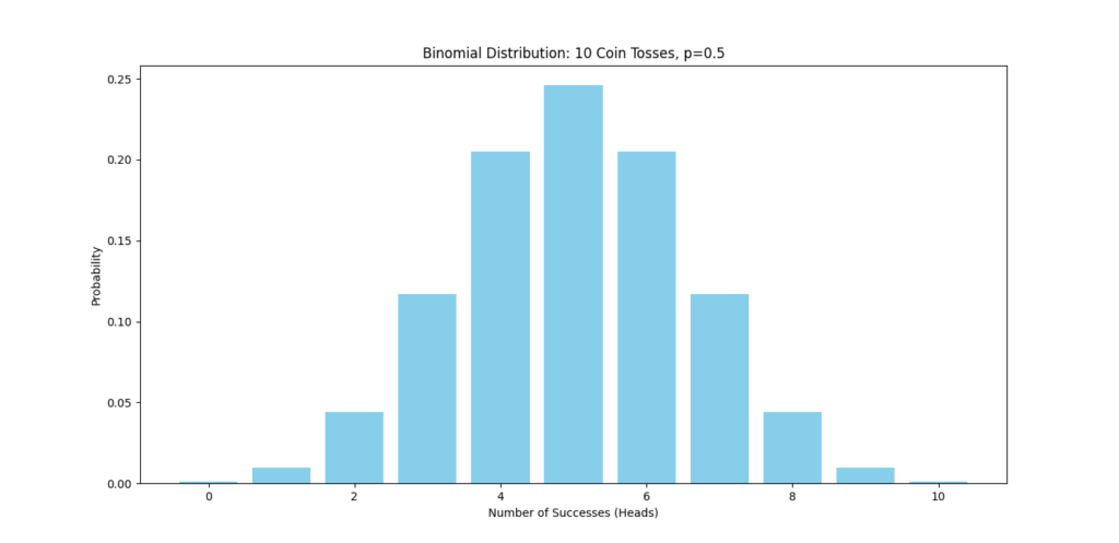
Now, let’s look at how likely it is to get different numbers of heads (from 0 to 10) when tossing a coin 10 times. We’ll plot the probabilities using Matplotlib.
Applications in Machine Learning and A/B Testing
1. A/B Testing Example
Let’s say this taht we have two versions of a website, Version A and Version B. We want to know if users are more likely to click on Version B. Let’s say Version B has been tested with 50 users, and 30 of them clicked on it. If we assume a baseline click probability of 0.5 (random chance), we can use the binomial distribution to test if our result is statistically significant.
Here’s how to calculate it in Python:
# A/B testing example parameters
n = 50      # Number of users shown Version B
k = 30      # Number of clicks
p = 0.5     # Baseline probability of a click

# Calculate the probability of getting exactly 30 clicks if the baseline is true
probability = binom.pmf(k, n, p)
print(f"Probability of getting exactly {k} clicks out of {n} is: {probability:.4f}")
2. Machine Learning Example
In classification tasks, the binomial distribution can help evaluate the model’s accuracy. For instance, if a spam classifier correctly identifies spam emails with a 95% success rate, we can use the binomial distribution to estimate the probability of correct classifications in the next 100 emails.
# Parameters for the classifier
n = 100     # Number of emails
p = 0.95    # Probability of correctly identifying spam

# Calculate probabilities for a range of correct identifications (from 90 to 100)
k_values = np.arange(90, n+1)
binomial_probabilities = binom.pmf(k_values, n, p)

# Print results
for k, prob in zip(k_values, binomial_probabilities):
    print(f"Probability of exactly {k} correct classifications: {prob:.4f}")
Summary Table: Key Points
| Scenario | Parameters | Calculation | Example in Data Science |
|---|---|---|---|
| Coin Toss (Success/Failure) | n=10,p=0.5 | Probability of 6 heads | Tossing a coin 10 times |
| A/B Testing | n=50,p=0.5 | Probability of 30 clicks | Testing if Version B has better engagement |
| Spam Classifier Accuracy | n=100,p=0.95 | Probability of correct classification | Predicting spam emails with 95% accuracy |
Poisson Distribution: Understanding Event Prediction and Rare Events
The Poisson distribution is a key concept in probability, especially useful for predicting the likelihood of rare events happening over a specific time frame or space. If you’ve ever been curious about estimating events like daily website visits, emails received, or calls at a support center, this distribution is for you. It helps us model situations where events occur independently and randomly, but we know the average rate (like 10 calls per hour).
In data science, the Poisson distribution is particularly valuable for tasks related to event prediction and rare event modeling.
What Is Poisson Distribution?
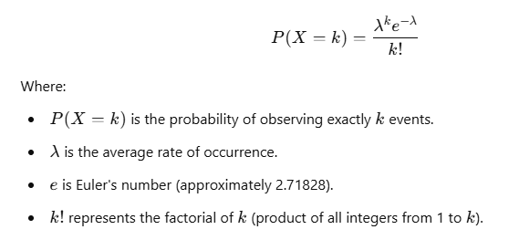
The Poisson distribution models the probability of observing k events within a fixed interval of time or space, given that events happen at a known average rate, λ (lambda). Here’s the mathematical formula:
Real-Life Example: Customer Calls at a Call Center
Let’s say a call center averages 3 calls per hour. If we want to know the probability of receiving exactly 5 calls in one hour, we can plug these values into the formula:
- λ=3 (average number of calls per hour)
- k=5 (exactly 5 calls in an hour)

This probability gives us insight into how often we might see a rare increase in calls beyond the average.
Applications of Poisson Distribution in Data Science
1. Event Prediction:
- When dealing with events that occur randomly but at a consistent average rate, like server requests per minute or defect reports per day, the Poisson distribution helps data scientists estimate the probability of specific outcomes.
2. Rare Event Modeling:
- In fields like insurance, healthcare, and fraud detection, identifying rare but critical events—such as car accidents, disease outbreaks, or unusual financial transactions—can benefit from Poisson modeling.
Using Python to Calculate Poisson Probabilities
Let’s calculate the probability of receiving exactly 5 calls in one hour for our call center example using Python.
from scipy.stats import poisson

# Parameters
lambda_rate = 3   # Average rate (3 calls per hour)
k = 5             # Desired number of calls

# Calculate Poisson probability
probability = poisson.pmf(k, lambda_rate)
print(f"The probability of receiving exactly {k} calls in one hour is: {probability:.4f}")
Visualizing the Poisson Distribution
To see the spread of possible outcomes, we can plot the Poisson distribution for different numbers of calls in an hour, given an average rate of 3.
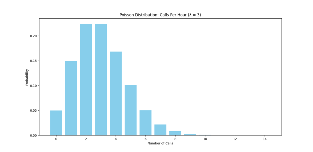
This plot will show the probabilities for receiving between 0 and 15 calls in an hour, helping us visualize likely and unlikely scenarios.
Use Cases of Poisson Distribution in Data Science
1. Website Traffic Analysis
- Suppose a website averages 200 visits per day. The Poisson distribution can help estimate the probability of receiving exactly, say, 250 visits on a given day, which could indicate a spike in interest or an issue.
2. Predicting Equipment Failures
- Manufacturing companies often use Poisson models to predict the likelihood of machine breakdowns in a month. If a particular machine fails about 2 times a month on average, the Poisson distribution can help assess the chances of more frequent failures, which could inform maintenance schedules.
3. Healthcare: Modeling Patient Arrivals
- In emergency rooms, it’s useful to predict patient arrival rates. If an ER typically sees 10 patients per hour, the Poisson distribution helps assess busy periods by modeling probabilities for various arrival rates (e.g., 15 patients in an hour).
4. Finance: Fraud Detection
- In banking, the Poisson distribution can help identify unusual transaction patterns. If a typical account sees one transfer per day, a sudden spike of 10 transfers could trigger a fraud alert.
Summary Table: Key Points for Poisson Distribution
| Scenario | Parameters | Calculation | Example in Data Science |
|---|---|---|---|
| Call Center Calls | λ=3 | Probability of 5 calls | Estimating busy call hours |
| Website Visits | λ=200 | Probability of 250 visits | Detecting traffic surges |
| Machine Failures | λ=2 | Probability of breakdowns | Planning maintenance schedules |
| ER Patient Arrivals | λ=10 | Probability of 15 arrivals | Managing hospital resources |
| Banking Fraud Detection | λ=1 | Probability of high transfers | Identifying suspicious activities |
Geometric Distribution: Understanding Success and Failure Predictions
The geometric distribution is a powerful tool in probability theory. It helps us understand the number of trials needed until the first success in a series of independent experiments. This concept can be quite useful in various fields, including data analysis and machine learning.
Imagine you’re tossing a coin and want to know how many tosses it takes until you get your first head. The geometric distribution gives us a way to predict that! It’s all about counting how many tries it takes before achieving that first success.
Introduction to Geometric Distribution
In simple terms, the geometric distribution deals with “success” and “failure” in repeated trials. The key characteristics include:
- Trials are independent: The outcome of one trial doesn’t affect another.
- Two possible outcomes: Each trial results in either success (like getting heads) or failure (like getting tails).
- Constant probability: The chance of success remains the same for each trial.
The mathematical formula for the geometric distribution is:
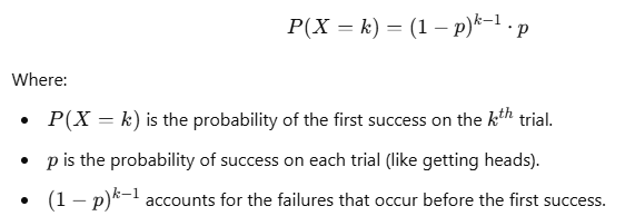
Real-Life Example: Coin Tossing
Let’s say you flip a coin, and the chance of getting heads (success) is 0.5. You want to find out the probability of getting your first head on the third toss.
Using our formula:
- p=0.5
- k=3
The probability calculation would look like this:

So, there’s a 12.5% chance that you’ll get your first head on the third toss.
How Geometric Distribution Helps in Predicting Successes and Failures
The geometric distribution is especially useful in situations where we want to predict how many attempts it will take to achieve the first success. Here are a few applications:
1. Marketing Campaigns:
- Businesses can use the geometric distribution to estimate how many customer contacts are needed before making the first sale. If the chance of converting a lead into a sale is 20%, companies can predict sales outcomes based on this distribution.
2. Quality Control:
- In manufacturing, the geometric distribution can help assess the number of products tested before finding the first defect. If the defect rate is low, knowing how many products might need to be checked can improve quality assurance processes.
3. Sports Analytics:
- Coaches might analyze how many attempts it takes a player to score their first goal in a game, helping with strategies and training focus.
4. Call Centers:
- In customer service, the geometric distribution can predict the number of calls an agent might handle before resolving a customer’s issue.
Visualizing the Geometric Distribution
Let’s use Python to visualize the geometric distribution for different probabilities of success. We’ll show how the probability changes with the number of trials until the first success.
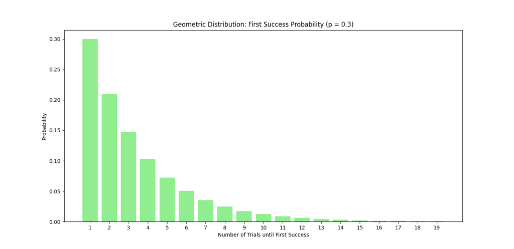
This plot will display how likely it is to achieve the first success over a series of trials, making it easy to understand the relationship between attempts and success.
Summary Table: Key Points for Geometric Distribution
| Scenario | Parameters | Calculation | Example in Data Analysis |
|---|---|---|---|
| Coin Tossing | p=0.5 (50% chance) | Probability of first heads on k tosses | Predicting how many tosses for a first head |
| Sales Conversion | p=0.2 (20% chance) | Probability of first sale after k contacts | Estimating customer outreach efforts |
| Quality Control | p=0.01 (1% chance) | Probability of first defect in products | Assessing product quality processes |
| Player Scoring | p=0.25 (25% chance) | Probability of first goal after k attempts | Evaluating player performance |
| Call Center | p=0.6 (60% chance) | Probability of first resolved call | Managing customer service interactions |
Must Read
- How to Diagnose Overfitting in Machine Learning — 9 Proven Tools
- PyTorch Debugging Checklist: A Systematic Framework to Fix Models That Won’t Learn
- Why sorted() Is Safer Than list.sort() in Production Python Systems
- Monotonic Sequence in Python: 7 Practical Methods With Edge Cases, Interview Tips, and Performance Analysis
- How to Check if Dictionary Values Are Sorted in Python
Continuous Probability Distributions: Understanding Their Role in Data Science
When we discuss continuous probability distributions, we’re exploring a part of statistics that helps us understand data that can take any value within a certain range. Unlike discrete distributions, which deal with countable outcomes (like counting how many cars pass a street), continuous distributions are used for data that can have infinite precision. Examples include measurements like height, weight, or time, where values can be as specific as needed.
Understanding Continuous Probability Distributions
A continuous probability distribution describes the probabilities of the possible values of a continuous random variable. Here are the key features:
- Range of Values: Continuous variables can take any value within a certain range. For example, someone’s height could be 170.1 cm, 170.2 cm, or 170.3 cm, and so on.
- Probability Density Function (PDF): The probability is represented using a function known as the probability density function. Unlike discrete distributions, where you calculate probabilities at specific points, in continuous distributions, the area under the curve represents probabilities.
- Cumulative Distribution Function (CDF): This function tells us the probability that a random variable is less than or equal to a certain value. It’s the integral of the PDF.
Mathematical Representation
For a continuous random variable X with a PDF f(x), the probability that X lies within an interval [a,b] is given by:

Real-Life Applications of Continuous Distributions in Data Science
Continuous probability distributions are used in various fields, and understanding them is crucial for data scientists. Here are some real-life applications:
1. Modeling Heights and Weights:
- In a study of human heights, we might use a normal distribution (a common continuous distribution) to represent the average height of a population. By understanding the distribution, researchers can make predictions about the likelihood of individuals falling within certain height ranges.
2. Time to Complete Tasks:
- In project management, the time required to complete tasks often follows a continuous distribution. For example, if the average time to finish a software development task is 10 hours, the actual time may vary. Using continuous distributions helps project managers estimate the probability of completing a task within a certain timeframe.
3. Financial Modeling:
- In finance, asset returns are often modeled using continuous distributions like the normal distribution. By understanding how returns are distributed, investors can make better decisions regarding risk and investment strategies.
4. Quality Control:
- Manufacturers use continuous distributions to monitor the quality of products. For instance, if the weight of a packaged product is supposed to be 500 grams, a normal distribution can help determine how much variability is acceptable and how often products fall outside the desired weight range.
5. Machine Learning:
- Continuous probability distributions are essential in many machine learning algorithms. For example, in Gaussian Naive Bayes, the algorithm assumes that the features follow a normal distribution. Understanding these distributions can improve model accuracy and performance.
Visualizing Continuous Probability Distributions
Let’s look at how we can visualize a continuous distribution using Python. We’ll plot a normal distribution, which is one of the most common continuous distributions.

This graph of the normal distribution, showing how probabilities are distributed around the mean.
Summary Table: Key Points for Continuous Probability Distributions
| Scenario | Example | Distribution Used | Application in Data Science |
|---|---|---|---|
| Heights and Weights | Modeling average height | Normal Distribution | Estimating the range of heights |
| Task Completion Time | Software development tasks | Exponential Distribution | Estimating completion time probabilities |
| Financial Modeling | Asset return analysis | Normal Distribution | Understanding risk in investments |
| Quality Control | Monitoring packaged weights | Normal Distribution | Ensuring product quality |
| Machine Learning | Feature analysis | Gaussian Distribution | Improving model predictions |
Normal Distribution (Gaussian Distribution): A Key Concept in Data Science
What Is Normal Distribution and Why It Matters in Data Science?
The normal distribution, often called the Gaussian distribution, is a fundamental concept in statistics and data science. It describes how data points are spread out around a central mean. You’ve likely seen the classic bell-shaped curve, which visually represents a normal distribution.
Key Characteristics:
- Symmetry: The curve is symmetrical around the mean, meaning most data points cluster near the center, with fewer points appearing as you move away from the mean.
- Mean, Median, and Mode: In a normal distribution, these three measures of central tendency are equal and occur at the peak of the curve.
- Standard Deviation (σ): This measures the spread of the data points. A smaller standard deviation means data points are closer to the mean, while a larger standard deviation indicates more variability.
The importance of normal distribution in data science cannot be overstated. Many statistical methods and machine learning algorithms assume that data is normally distributed. This assumption allows for easier analysis and more accurate predictions.
Mathematical Representation of Normal Distribution
The normal distribution is mathematically represented by the probability density function (PDF):
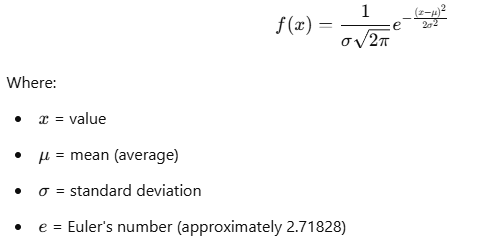
This formula describes how the probability of a random variable xxx is distributed in relation to the mean and standard deviation.
Applications in Predictive Modeling and Machine Learning
The normal distribution is crucial in various aspects of predictive modeling and machine learning. Here’s how:
- Feature Scaling:
- In many machine learning algorithms, it’s essential to standardize features so they follow a normal distribution. One common method is z-score normalization, which transforms data into a standard normal distribution with a mean of 0 and a standard deviation of 1.
Python Code Example:
import numpy as np

# Sample data
data = np.array([10, 20, 30, 40, 50])
mean = np.mean(data)
std_dev = np.std(data)

# Z-score normalization
z_scores = (data - mean) / std_dev
print("Z-scores:", z_scores)
2. Assumptions in Algorithms:
- Many algorithms, such as linear regression, assume that the residuals (the differences between observed and predicted values) follow a normal distribution. This assumption allows for better predictions.
3. Hypothesis Testing:
- In statistics, many hypothesis tests rely on the assumption that data follows a normal distribution. This assumption is crucial for determining whether there is a significant difference between groups.
4. Anomaly Detection:
- Normal distribution helps identify anomalies. If you expect a measurement to follow a normal distribution, any value far from the mean can be flagged as unusual.
5. Confidence Intervals:
- When estimating population parameters, the normal distribution is used to create confidence intervals. This provides a range of values within which we can expect a population parameter to lie with a certain level of confidence.
Advantages of Using Normal Distribution in Data Science
The normal distribution offers several benefits, making it a preferred choice in data science:
- Simplicity: Its mathematical properties make it easier to work with than other distributions.
- Predictability: Many statistical methods are built on the assumption of normality, providing a reliable framework for analysis.
- Central Limit Theorem: This theorem states that regardless of the original population’s distribution, the sampling distribution of the sample mean will tend to be normal if the sample size is large enough.
Summary Table: Key Points of Normal Distribution
| Feature | Description |
|---|---|
| Shape | Bell-shaped curve, symmetrical around the mean |
| Central Tendency | Mean, median, and mode are equal |
| Standard Deviation | Measures spread; influences the width of the curve |
| Applications | Used in feature scaling, regression models, and hypothesis testing |
| Advantages | Simplicity, predictability, and reliance on the Central Limit Theorem |
Uniform Distribution: A Simple and Essential Concept in Data Science
Overview of Uniform Distribution in Data Science
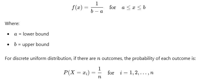
Uniform distribution is a fundamental probability distribution in statistics. It describes a scenario where all outcomes are equally likely to occur within a specified range. Imagine a fair die: each number (1 through 6) has the same chance of being rolled. This is a perfect example of a uniform distribution.
Key Characteristics:
- Equal Probability: Every value in the range has the same probability of occurring.
- Continuous vs. Discrete: Uniform distribution can be either continuous (infinite possibilities within a range) or discrete (finite outcomes).
In a continuous uniform distribution, the probability density function (PDF) is represented as:
When and Where to Use Uniform Distribution in Data Science
Uniform distribution is widely used in various applications within data science. Here are some key scenarios where it is applicable:
- Random Sampling:
- When selecting a sample from a population, uniform distribution ensures that every individual has an equal chance of being selected. This approach helps eliminate bias in the sampling process.
import numpy as np

# Generate 10 random samples from a uniform distribution between 1 and 10
samples = np.random.uniform(1, 10, 10)
print("Random Samples from Uniform Distribution:", samples)
2. Simulations:
- In simulations, uniform distribution is often used to generate random numbers. For instance, in Monte Carlo simulations, uniform random numbers are used to model complex systems.
3. Game Development:
- In video games, uniform distribution can determine the spawn rates of items or characters. For example, if a player has an equal chance of finding any item in a treasure chest, that distribution can be modeled as uniform.
4. Quality Control:
- In manufacturing, uniform distribution can model the tolerance levels for parts. If all outcomes within a specific range are acceptable, it reflects a uniform distribution.
5. A/B Testing:
- Uniform distribution helps in A/B testing scenarios by randomly assigning users to different groups, ensuring that each group has an equal chance of receiving different treatments or versions.
Visualizing Uniform Distribution with Python
To better understand the uniform distribution, let’s visualize it using Python. The following code creates a plot of a continuous uniform distribution.
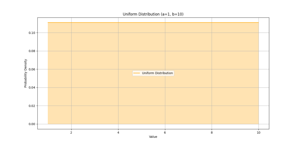
This visual representation of the uniform distribution, showing that every value within the range [1, 10] has the same probability density.
Summary Table: Key Points of Uniform Distribution
| Feature | Description |
|---|---|
| Shape | A flat line representing equal probability across the range |
| Probability | Each outcome has an equal chance of occurring |
| Applications | Used in random sampling, simulations, quality control, and A/B testing |
| Continuous vs. Discrete | Can be either continuous (infinite possibilities) or discrete (finite outcomes) |
Exponential Distribution: Understanding Time and Predictability in Data Science
Introduction to Exponential Distribution
Exponential distribution is a probability distribution that describes the time between events in a process where events happen continuously and independently at a constant average rate. It’s commonly used in various fields, including data science, to model time until an event occurs.
Think of it this way: if you’re waiting for a bus that comes every 10 minutes on average, the time you wait can be modeled using an exponential distribution. Sometimes you may catch the bus right away, and other times you might wait longer, but the average waiting time remains constant.
Key Characteristics of Exponential Distribution:
- Memoryless Property: The future is independent of the past. For example, if you’ve waited for 5 minutes already, the time you wait now doesn’t depend on those 5 minutes.
- Continuous Distribution: Exponential distribution applies to continuous outcomes, meaning it can take any positive value.
The probability density function (PDF) for the exponential distribution is given by:

Where:
- λ = rate parameter (average rate of events)
- x = time until the event occurs
How Exponential Distribution Affects Time-Based Predictions in Data Science
Exponential distribution is particularly useful for modeling time-related data. Here’s how it plays a role in various applications within data science:
- Modeling Time Until Events:
In reliability engineering, the exponential distribution is often used to model the time until a device fails. For instance, if a light bulb has an average lifetime of 1000 hours, you can predict the probability of it burning out after a certain number of hours.
2. Queueing Theory:
Exponential distribution is fundamental in analyzing waiting times in queues. For example, in a restaurant, you can predict how long a customer will wait for service based on the average rate of customers being served.
3. Survival Analysis:
In healthcare, exponential distribution helps estimate the time until an event occurs, such as the time until a patient experiences a relapse.
When analyzing time-series data, the exponential distribution can assist in modeling the duration of events over time, making it easier to identify trends and make predictions.
5. Predictive Maintenance:
In manufacturing, knowing when machines are likely to fail can help schedule maintenance and prevent downtime. The exponential distribution aids in predicting these failure times.
Visualizing Exponential Distribution with Python
To understand the exponential distribution better, let’s visualize it using Python. The following code generates and plots an exponential distribution.
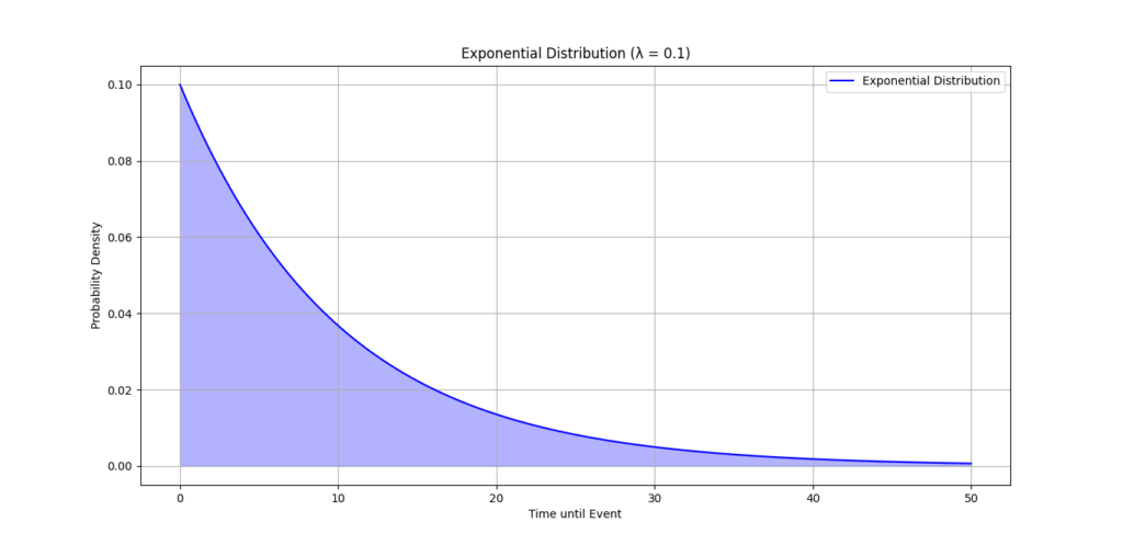
This visualizes the exponential distribution, showing how the probability of waiting time decreases as time increases.
Summary Table: Key Points of Exponential Distribution
| Feature | Description |
|---|---|
| Shape | A curve that starts high and decreases as time increases |
| Memoryless | The future wait time is independent of the past |
| Applications | Used in reliability analysis, queueing theory, and survival analysis |
| Continuous Distribution | Applies to time until events (e.g., failure times) |
Log-Normal Distribution: Understanding Skewness in Machine Learning
What is the Log-Normal Distribution?
A log-normal distribution is a probability distribution of a random variable whose logarithm is normally distributed. This means if you take the natural logarithm of a log-normally distributed variable, the result will be normally distributed.
In simpler terms, if you have data that are always positive and tend to cluster around a certain value, but can also have some larger values (like income, stock prices, or certain biological measurements), that data might follow a log-normal distribution.
Key Characteristics of Log-Normal Distribution:
- Asymmetry: Unlike the normal distribution, which is symmetric, a log-normal distribution is skewed to the right. This means there are more small values and a few very large ones.
- Positive Values Only: Log-normal distribution is defined for values greater than zero.
The probability density function (PDF) for the log-normal distribution is given by:

Where:
- μ\muμ = mean of the natural logarithm of the variable
- σ\sigmaσ = standard deviation of the natural logarithm of the variable
Use Cases for Log-Normal Distribution in Predicting Skewed Data
Log-normal distribution has several important applications in machine learning and data analysis, particularly for predicting skewed data:
- Financial Data:
- Stock prices and income distributions often follow a log-normal distribution. For example, while most people earn a modest salary, a few may earn significantly more, leading to a right-skewed income distribution.
- Environmental Data:
- Measurements such as pollutant concentrations or the size of particles in a material can also be modeled using a log-normal distribution, as they tend to cluster around lower values with a few outliers.
- Biological Measurements:
- Certain biological measurements, like the size of organisms or the concentration of a substance in a sample, often fit a log-normal distribution because of the multiplicative processes in nature.
- Predicting Sales:
- In business, sales data for products can often be skewed, with most products selling a small number of units, while a few sell exceptionally well. Understanding this distribution can help in forecasting sales more accurately.
- Machine Learning Applications:
- When building predictive models, recognizing that your target variable follows a log-normal distribution can help in choosing the right algorithms and transformations. For instance, applying a logarithmic transformation to the target variable before training a model can improve predictions.
Visualizing Log-Normal Distribution with Python
To visualize how a log-normal distribution looks, let’s create a plot using Python.
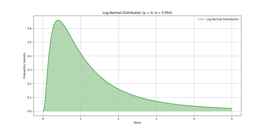
This log-normal distribution illustrates how most of the values are clustered towards the lower end, with some extending to higher values.
Summary Table: Key Points of Log-Normal Distribution
| Feature | Description |
|---|---|
| Shape | Right-skewed distribution with a long tail on the right |
| Values | Defined only for positive values |
| Applications | Commonly used in finance, environmental science, and biology |
| Machine Learning Use | Useful for predicting skewed data and improving model accuracy |
Conclusion: The Impact of Probability Distributions on Data Science Success
As we wrap up our discussion on probability distributions, it’s clear that they play a crucial role in data science. Understanding these distributions helps us make sense of data and guides us in making informed decisions.
Recap of Key Points on Probability Distributions
Throughout this exploration, we’ve covered several essential concepts related to probability distributions:
- Types of Distributions: We examined both discrete and continuous distributions, including important types like the binomial, Poisson, normal, and log-normal distributions. Each type has its own characteristics and applications.
- Real-World Applications: We highlighted how probability distributions are used in various fields, from finance to environmental science, demonstrating their wide-ranging impact on real-life situations.
- Statistical Modeling: Mastering probability distributions enhances your ability to build predictive models. By understanding the underlying distribution of your data, you can choose the right models and techniques for analysis.
How Mastery of Probability Distributions Can Boost Data Science Skills
When you have a solid grasp of probability distributions, your data science skills improve significantly. Here’s how:
- Enhanced Data Analysis: You’ll be better equipped to analyze data patterns and behaviors, leading to more accurate insights and predictions.
- Informed Decision-Making: Knowing how to apply different distributions allows you to make informed decisions based on statistical evidence rather than guesswork.
- Improved Model Performance: By selecting appropriate models based on the distribution of your data, you can enhance the accuracy and reliability of your machine learning algorithms.
Mastering probability distributions is not just about crunching numbers; it’s about understanding the stories behind the data. This knowledge can give you a competitive edge in your career.
External Resources
Probability and Statistics for Data Science
- This course covers the basics of probability and statistics, focusing on how these concepts apply to data science, including various probability distributions.
- Link to Course
edX: “Probability – The Science of Uncertainty and Data” by MIT
- This course offers an in-depth look at probability theory and its applications, including different types of probability distributions.
- Link to Course
FAQs
What Are Probability Distributions?
Probability distributions describe how the values of a random variable are spread out. They indicate the likelihood of different outcomes occurring, helping us understand the behavior of data.
Why Are Probability Distributions Important in Data Science?
Probability distributions are crucial because they provide the foundation for statistical analysis. They help data scientists model uncertainty, make predictions, and draw conclusions from data, which informs decision-making.
Which Probability Distributions Are Commonly Used in Data Science?
Commonly used probability distributions include:
Exponential Distribution: Commonly applied in time-to-event data.
Normal Distribution: Often used in predictive modeling.
Binomial Distribution: Useful for binary outcomes, like success or failure.
Poisson Distribution: Ideal for counting events in fixed intervals.
How Do I Choose the Right Probability Distribution for My Data?
To choose the right probability distribution, consider the following:
Statistical Tests: Use tests like the Chi-square goodness-of-fit test to assess how well a distribution fits your data.
Type of Data: Determine if your data is discrete (countable) or continuous (measurable).
Data Characteristics: Analyze the shape of your data. For example, is it symmetric or skewed?
Context of Use: Think about the real-world scenario you’re modeling. Some distributions fit specific situations better than others.



Leave a Reply