Basic Probability for Data Science with examples: A Complete Guide
Introduction to Basic Probability for Data Science
If you’re enter into Data Science, understanding Probability for Data Science is a must. It’s the foundation behind so many things, from predicting outcomes to making informed decisions with data. But don’t worry—this guide will walk you through the basics.
We’ll cover the most important ideas, like what probability is, how to calculate it, and how it applies to data science. You’ll see how concepts like random events, probability distributions, and independent events fit into the bigger picture of analyzing data and building models.
Whether you’re new to data science or just need a refresher, this guide is for you. By the end, you’ll have a solid understanding of probability and how to use it in real-world data science problems. Let’s get started!
What Is Probability in Data Science?
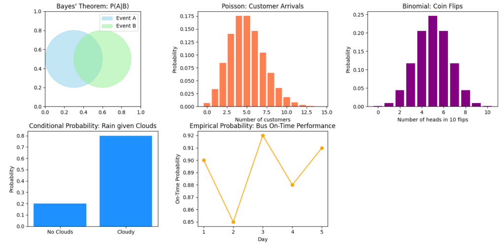
Here is a visualization of key probability concepts commonly used in data science:
- Bayes’ Theorem (Top Left): Represented by two overlapping circles (events A and B), showcasing conditional probability.
- Poisson Distribution (Top Center): A bar graph representing customer arrival probabilities based on an average rate (λ=5).
- Binomial Distribution (Top Right): Visualizing the probability of getting a specific number of heads in 10 coin flips.
- Conditional Probability (Bottom Left): A bar graph showing the probability of rain given the presence of clouds.
- Empirical Probability (Bottom Center): A line plot showing the probability of buses arriving on time over five days.
These concepts provide a foundation for making predictions and understanding patterns in data science.
Let’s talk about probability—something we all use every day without even realizing it. Whether you’re predicting the weather or guessing how long your commute will take, you’re working with probability. In data science, probability plays a huge role in helping us understand and make predictions from data. It’s the tool we use to deal with uncertainty, and trust me, there’s always a lot of that when working with data!
So why does probability matter so much in data science? Well, when we look at a dataset, it’s almost impossible to know what’s going to happen with complete certainty. That’s where probability comes in. It helps us estimate outcomes, make predictions, and even build machine learning models. Without probability, we’d be guessing blindly.
Why Probability Is Important in Data Science
One of the main reasons probability for data science is important is because it lets us make informed decisions. For instance, when you’re training a machine learning model to predict whether an email is spam, the model isn’t 100% sure. Instead, it’s calculating the probability that an email is spam based on what it learned from the data. If that probability is high enough, the email gets marked as spam.
Think about it this way: the weather forecast you check every morning is based on probability. The meteorologist doesn’t know for sure it’s going to rain, but they look at data and say, “There’s a 70% chance.” In the same way, data scientists use probability to predict things like whether a customer will buy a product or how much traffic a website will get.
Here’s a breakdown of why probability matters so much in data science:
- Predicting outcomes: Machine learning models use probability to predict outcomes. For example, if you’re using a model to classify whether an image contains a cat or a dog, the model will estimate the probability of each.
- Dealing with uncertainty: Data is rarely perfect. Probability helps us handle the uncertainty that comes with missing data, random events, and unpredictable outcomes.
- Modeling randomness: Many real-world problems are influenced by random factors, and probability allows us to model these random events accurately.
Basic Probability Concepts You Need to Know
Let’s go over some of the basic probability concepts that you’ll often see in data science:
- Random Variables:
- A random variable is just a fancy way of saying something that can take on different outcomes.
- Example: Think of rolling a die. The result—whether it’s a 1, 2, 3, 4, 5, or 6—is a random variable.
- Probability Distributions:
- This is how we describe the likelihood of different outcomes. The most famous one is the normal distribution, which is that classic bell curve shape.
- Example: Heights of people usually follow a normal distribution, where most people are around the average height, and fewer are extremely tall or short.
- Conditional Probability:
- This is the probability of something happening given that something else has already happened.
- Example: If you know someone bought a phone, you might want to know the probability they’ll also buy a phone case. That’s conditional probability.
- Bayes’ Theorem:
- Bayes’ Theorem helps us update our predictions when new information comes in.
- Example: In medical testing, if a person tests positive for a disease, Bayes’ Theorem helps us calculate how likely it is that they actually have the disease, based on the accuracy of the test and the overall likelihood of the disease.
- Independent Events:
- Independent events are those that don’t affect each other.
- Example: Tossing a coin twice. The result of the first toss doesn’t change the result of the second.
Real-Life Applications of Probability in Data Science
Now, how does this all work in real life? Let’s look at some ways probability is used in data science:
- Spam Detection: Many email services use probability-based algorithms to detect spam. They analyze the words in an email and estimate how likely it is to be spam.
- Customer Behavior Prediction: E-commerce sites use probability to predict what products you might buy next, based on your previous purchases.
- Stock Market Analysis: Analysts use probability models to forecast stock prices, factoring in past performance and market conditions.
Here’s a simple Python example to show how probability for data science works in action:
from sklearn.naive_bayes import GaussianNB
from sklearn.model_selection import train_test_split
from sklearn.datasets import load_iris

# Load dataset
data = load_iris()
X_train, X_test, y_train, y_test = train_test_split(data.data, data.target, test_size=0.3)

# Gaussian Naive Bayes model
model = GaussianNB()
model.fit(X_train, y_train)

# Predict on test set
predictions = model.predict(X_test)
print(predictions)
In this code, we’re using the Naive Bayes algorithm—which is based on probability—to classify the famous Iris dataset.
Quick Summary of Probability Concepts
To make things clearer, here’s a simple table to summarize the key concepts we’ve talked about:
| Concept | Definition | Example |
|---|---|---|
| Random Variables | Variables that represent random outcomes | Rolling a die |
| Probability Distribution | Describes how probabilities are spread over outcomes | Heights, test scores |
| Conditional Probability | Probability of an event given another event has occurred | Buying a phone case after buying a phone |
| Independent Events | Events that don’t affect each other | Tossing a coin twice |
| Bayes’ Theorem | Updates the probability of a hypothesis as more evidence is available | Medical test results |
Basic Concepts of Probability
Random Variables
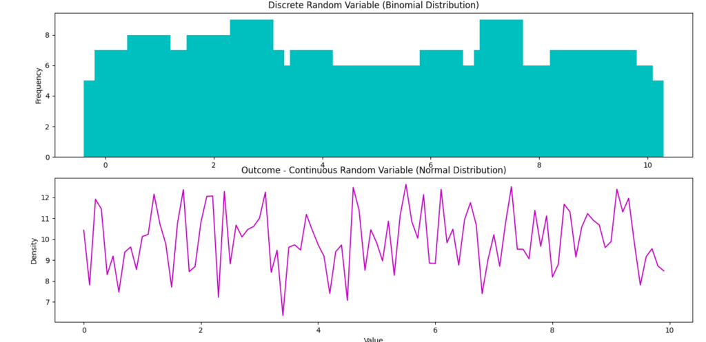
In simple terms, a random variable is quantify the outcomes of random events. When you roll a die, the result can be any number from 1 to 6. This number is what we call a random variable because it can change with each roll.
Understanding Random Variables in Data Science
In data science, random variables are crucial because they help us model and analyze real-world situations that involve uncertainty. They come in two main types: discrete and continuous.
- Discrete Random Variables: These take on specific, separate values. For example, the number of people in a room can only be a whole number (0, 1, 2, 3, etc.). If we were to analyze data on how many products a customer buys, that number would also be discrete.
- Continuous Random Variables: These can take on any value within a range. Think of measurements like height or weight. If we measure the height of students, it could be any value within a given range, such as 150.5 cm.
Example in Data Science
You are working on a project predicting customer purchases based on past behavior. Here, the random variable might be the number of items a customer buys in a single transaction. If you analyze this data, you can use it to calculate probabilities of different purchase amounts, allowing you to customize marketing strategies effectively.
import numpy as np
import matplotlib.pyplot as plt

# Simulating a discrete random variable (number of purchases)
purchases = np.random.poisson(lam=3, size=1000)

# Plotting the distribution of purchases
plt.hist(purchases, bins=range(10), alpha=0.7, color='blue', edgecolor='black')
plt.title('Distribution of Customer Purchases')
plt.xlabel('Number of Purchases')
plt.ylabel('Frequency')
plt.show()
In this code snippet, we simulate the number of purchases using a Poisson distribution, which is often used for counting events.
Events in Probability
Now that we’ve covered random variables, let’s discuss events. In the context of data science, an event is simply a specific outcome or a collection of outcomes from a random experiment.
Event Definition in Probability Theory
Here’s a simple way to understand it: if we consider flipping a coin, the possible outcomes are heads or tails. If we define the event as “getting heads,” we are focusing on one specific outcome.
Event Probability
Every event has a probability associated with it, which tells us how likely that event is to happen. Probability is a number between 0 and 1, where 0 means the event will not happen, and 1 means it will definitely happen.
- Example of Events:
- Event A: Rolling a 4 on a die.
- Event B: Choosing a red card from a deck of cards.
To calculate the probability of Event A, we would use the formula:

Probability Distribution
Next, let’s talk about probability distributions. This concept is vital in data science because it allows us to understand how probabilities are distributed across different outcomes.
Different Types of Probability Distributions in Data Science
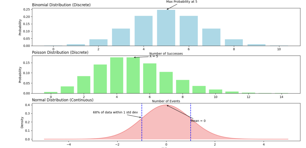
A probability distribution describes how the probabilities of a random variable are allocated across its possible values. There are two main types:
- Discrete Probability Distributions: Used for discrete random variables. An example is the Binomial distribution, which models the number of successes in a fixed number of trials, such as flipping a coin multiple times.
- Continuous Probability Distributions: Used for continuous random variables. An example is the Normal distribution (bell curve), which is common in natural phenomena like heights, test scores, etc.
Why Probability Distributions Matter
Understanding these distributions is crucial for data analysis and modeling because they provide insights into the behavior of data. Here’s why:
- Modeling Data: They help us model real-world phenomena accurately.
- Making Predictions: Probability distributions allow us to make predictions about future events based on historical data.
- Statistical Inference: They are the foundation for making inferences about populations based on sample data.
A Quick Table of Common Probability Distributions
| Type | Distribution Name | Use Case |
|---|---|---|
| Discrete | Binomial | Number of successes in a series of trials |
| Discrete | Poisson | Number of events in a fixed interval |
| Continuous | Normal | Heights, test scores, many natural phenomena |
| Continuous | Exponential | Time until an event occurs (e.g., failures) |
Must Read
- PyTorch Debugging Checklist: A Systematic Framework to Fix Models That Won’t Learn
- Why sorted() Is Safer Than list.sort() in Production Python Systems
- Monotonic Sequence in Python: 7 Practical Methods With Edge Cases, Interview Tips, and Performance Analysis
- How to Check if Dictionary Values Are Sorted in Python
- Check If a Tuple Is Sorted in Python — 5 Methods Explained
Types of Probability in Data Science
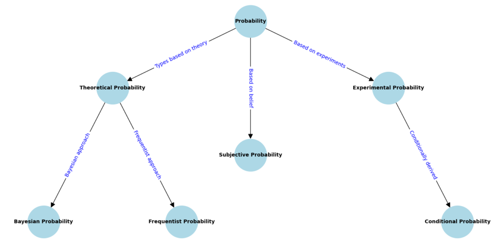
Classical Probability
Let’s talk about classical probability. This type of probability is all about the idea that you can predict the likelihood of an event happening based on all the possible outcomes in a fair situation. Think of it like rolling a fair die or flipping a fair coin.
Understanding Classical Probability
The formula for classical probability is:

Real-World Examples
- Rolling a Die: When rolling a standard six-sided die, the possible outcomes are {1, 2, 3, 4, 5, 6}. If you want to find the probability of rolling a 3, there is only one favorable outcome (rolling a 3) among six possible outcomes.

How to Calculate Classical Probability
Calculating classical probability involves a few simple steps:
- Identify the Event: Determine the event whose probability you want to calculate.
- Count the Favorable Outcomes: Figure out how many outcomes favor your event.
- Count the Total Outcomes: Count all possible outcomes in the situation.
- Apply the Formula: Use the classical probability formula to get your answer.
By following these steps, you can easily determine the probability of various events, which is crucial in fields like data science.
Empirical Probability
Now, let’s switch gears and explore empirical probability. Unlike classical probability, empirical probability is based on observed data rather than theoretical outcomes. This type of probability helps you understand how often an event occurs in real-world situations.
Understanding Empirical Probability
The formula for empirical probability is:

Real-World Data and Examples in Data Science
- Weather Forecasting: Imagine you want to find the probability of rain in your city. If it rained on 30 out of the last 100 days, you could calculate the empirical probability of rain as follows:

This tells you there’s a 30% chance of rain based on real observations.
Customer Behavior: Let’s say you’re analyzing customer purchases. If 150 out of 500 customers bought a specific product during a sale, you can calculate the probability of a customer buying that product as:

Empirical Probability with Examples in Data Science
In data science, empirical probability is invaluable. Here are a few key points to remember:
- Data-Driven Decisions: Empirical probability allows businesses to make informed decisions based on historical data. This can lead to more accurate predictions and effective strategies.
- Dynamic Analysis: As new data comes in, empirical probabilities can change. This flexibility makes them especially useful in dynamic environments like e-commerce and finance.
- Examples in Coding: Here’s a quick code snippet showing how to calculate empirical probability using Python:
import pandas as pd

# Sample data: a list of purchases (1 = bought, 0 = not bought)
purchases = [1, 0, 1, 1, 0, 1, 0, 0, 1, 1]

# Calculate empirical probability of buying
probability_of_buying = sum(purchases) / len(purchases)
print(f"Empirical Probability of Buying: {probability_of_buying:.2f}")
This code snippet calculates the empirical probability based on a simple list of customer purchases.
Conditional Probability in Data Science
Conditional Probability in Data Science
Let’s explore conditional probability. This concept is crucial in data science as it helps us understand the likelihood of an event occurring, given that another event has already occurred. Think of it like this: you want to know the probability of someone being a cat owner, given that they have a pet. This is where conditional probability shines.
Understanding Conditional Probability
The formula for conditional probability is:

This formula helps us get a clearer picture of how two events are related, which is essential in many areas of data science.
Examples Related to Data Science
- Customer Segmentation: Imagine you want to know the probability that a customer who purchased a smartphone also buys a phone case. If 200 customers bought smartphones, and 50 of them bought cases, the probability would be calculated as follows:
- Event A: Customer buys a case.
- Event B: Customer buys a smartphone.

2. Health Studies: In healthcare, conditional probability can help determine the risk of a disease. Suppose a health study shows that out of 1,000 patients, 100 have high cholesterol, and 30 of those also have heart disease. The probability of a patient having heart disease given that they have high cholesterol can be calculated like this:
- Event A: Patient has heart disease.
- Event B: Patient has high cholesterol.

How to Calculate Conditional Probability
Calculating conditional probability can be broken down into a few simple steps:
- Define Your Events: Clearly identify the two events you are interested in.
- Find Joint Probability: Determine the probability of both events occurring together.
- Find Marginal Probability: Calculate the probability of the conditioning event (the one you are conditioning on).
- Apply the Formula: Use the conditional probability formula to get your answer.
Example Calculation
Let’s say we want to find the conditional probability of a user engaging with an ad given they are in the age group of 18-25.
- Event A: User engages with the ad.
- Event B: User is aged 18-25.
Assume:
- 300 users engaged with the ad.
- 100 users are in the age group of 18-25.
- 50 users who are in that age group engaged with the ad.
Using the formula:

Conditional Probability in Machine Learning Models
Conditional probability plays a significant role in machine learning algorithms, particularly in models like the Naive Bayes classifier. This model uses conditional probability to make predictions about classifications.
How It Works
- Naive Bayes Classifier: This algorithm calculates the probability of a class label given a set of features. It assumes that all features are independent given the class label. The formula used is:
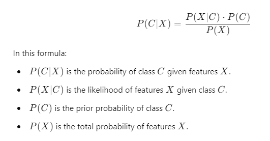
By using conditional probabilities, Naive Bayes can quickly classify data points based on past data, making it a popular choice for spam detection, sentiment analysis, and more.
Probability Distributions in Data Science
When it comes to Probability for Data Science, understanding probability distributions is essential. They provide a framework for modeling uncertainty and help us make informed predictions based on data. Let’s break down what probability distributions are, explore their types, and see how they apply in real-world scenarios.
What Are Probability Distributions?
A probability distribution describes how the probabilities of a random variable are distributed. In simpler terms, it tells us the likelihood of different outcomes of a random process. Probability distributions can be classified into two main types: discrete and continuous.
- Discrete Probability Distributions: These are used when the possible outcomes are distinct and countable. For instance, the number of heads when flipping a coin multiple times.
- Continuous Probability Distributions: These apply when the outcomes can take any value within a range. An example is the height of individuals in a population.
Types of Probability Distributions in Data Science with Examples:
- Discrete Distributions:
- Binomial Distribution: Used when there are two possible outcomes (success or failure) in a fixed number of trials. For example, flipping a coin 10 times and counting the number of heads.
- Poisson Distribution: Models the number of events occurring in a fixed interval of time or space. For instance, the number of emails received in an hour.
- Continuous Distributions:
- Normal Distribution: Often referred to as the bell curve, it describes data that clusters around a mean. Heights of individuals typically follow this distribution.
- Exponential Distribution: Used to model the time until an event occurs, such as the time between arrivals of customers at a store.
Common Probability Distributions Used in Data Science
Normal Distribution
The normal distribution is one of the most commonly used distributions in data science. It is symmetrical and characterized by its mean (average) and standard deviation (spread).
- Example: Let’s say you want to analyze the test scores of students in a class. If the scores are normally distributed, most students will score around the mean, with fewer students scoring very high or very low.
- Application in Data Science: Normal distribution is crucial for various statistical analyses, including hypothesis testing and regression analysis. Many machine learning algorithms assume that the data follows a normal distribution.
Long-Tail Keyword: Normal distribution in data science.
Binomial Distribution
The binomial distribution is used when there are two outcomes, like success or failure, across a fixed number of trials.
- Example: Suppose you are flipping a coin 10 times, and you want to calculate the probability of getting exactly 6 heads. The formula for the binomial distribution is:
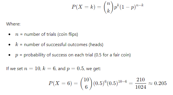
This means there’s about a 20.5% chance of getting exactly 6 heads in 10 flips.
Poisson Distribution
The Poisson distribution is used to model the number of times an event occurs in a given interval of time or space. This distribution is especially useful for rare events.
- Use Cases in Machine Learning and Data Science: Let’s say you are analyzing the number of customers arriving at a store every hour. If you know that, on average, 5 customers arrive each hour, you can use the Poisson distribution to predict the likelihood of 3 customers arriving in the next hour.
- Formula: The Poisson probability can be calculated using the formula:
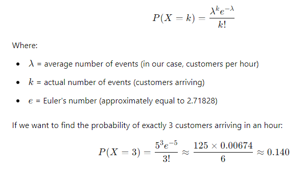
This indicates there’s about a 14% chance of having exactly 3 customers in that hour.
Probability Distributions in Data Science
Let’s break down probability distributions and why they’re so important for data science. These are basically tools that help us understand how data is spread out and what outcomes we can expect. If you’ve ever wondered how likely something is to happen, like a customer visiting your site, probability distributions help figure that out.
What Are Probability Distributions?
To put it simply, a probability distribution shows how likely different outcomes are. It tells us what values a variable can take and how often those values will show up.
There are two main types:
- Discrete probability distributions: These deal with countable outcomes, like the number of emails you get in a day.
- Continuous probability distributions: These apply to things that can take on any value, like the exact time it takes for a webpage to load.
Here’s a quick example. If you’re analyzing how long users spend on your website, that’s a continuous distribution because time can be 5.1, 5.15, or even 5.151 seconds. But if you’re counting how many users visit your site in a day, that’s a discrete distribution because you’ll get whole numbers (like 50 or 100 users).
Common Probability Distributions Used in Data Science
There are a few distributions you’ll run into a lot when working with data. Let’s go over the big ones.
Normal Distribution
You’ve probably heard of the normal distribution before—it’s also known as the bell curve. Most of the time, data clusters around a central point, which is the mean. For example, if you were to measure the heights of a group of people, most would be around the average height, and fewer would be either really tall or really short.
- Why it matters in data science: The normal distribution is everywhere! It’s used in things like predicting customer behavior or analyzing test scores. Let’s say you’re working on predicting sales. If your sales data follows a normal distribution, you can estimate how likely it is that next month’s sales will fall within a certain range.
Here’s how you can plot a normal distribution using Python:
import numpy as np
import matplotlib.pyplot as plt

data = np.random.normal(0, 1, 1000)  # Generate 1000 data points
plt.hist(data, bins=30, density=True)  # Create a histogram
plt.title("Normal Distribution")
plt.show()
Binomial Distribution
Now, let’s talk about the binomial distribution. This one’s perfect when you have a fixed number of trials, and each trial has two possible outcomes—success or failure. An easy example is flipping a coin. Every flip can either be heads or tails.
- How to use it in data science: Let’s say you want to know the probability of getting exactly 3 heads in 5 flips of a coin. The binomial distribution can help with that. Here’s a quick calculation:If ppp is the probability of success (getting heads), and nnn is the number of trials, the formula looks like this:

Poisson Distribution
The Poisson distribution is great for modeling rare events that happen over a certain amount of time or space. For instance, if you know that, on average, 10 people visit your site every hour, the Poisson distribution helps you figure out the chances of getting exactly 7 visitors in the next hour.
- Where it’s used: The Poisson distribution is useful in data science for things like predicting how often an event will happen, like the number of customer support tickets your team will get in a week.
Here’s how you can calculate it:
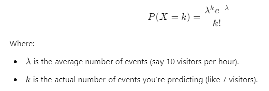
You can apply this to things like website traffic or predicting the number of calls to a help desk.
The Law of Large Numbers and Central Limit Theorem
What Is the Law of Large Numbers?
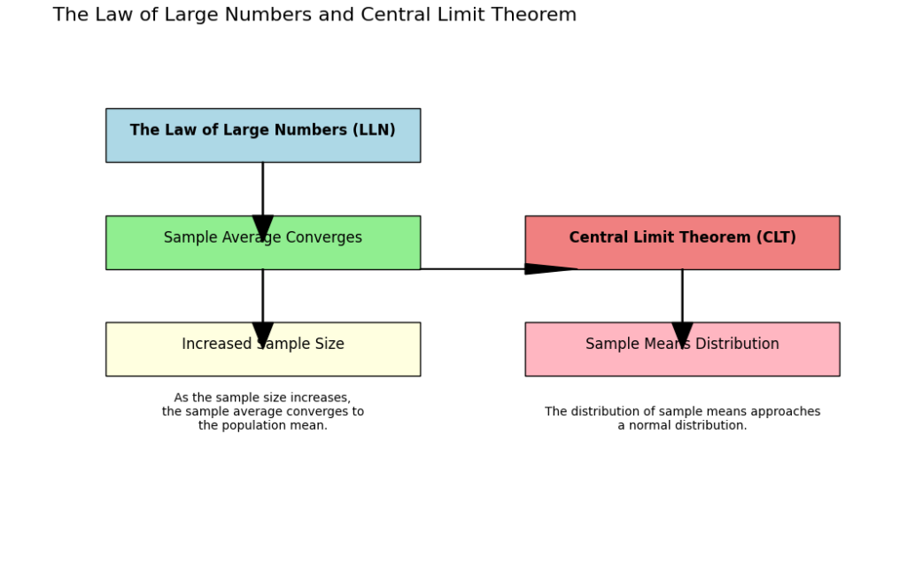
The Law of Large Numbers (LLN) is a core concept in probability for data science. In simple terms, this law tells us that as we collect more data or repeat an experiment many times, the average of the results will get closer to the expected value.
Let’s break it down with an example. Suppose you’re flipping a coin. The probability of getting heads is 50%. If you flip the coin 10 times, you might get 6 heads, or even 7, because the sample is small. But if you keep flipping the coin, say 1,000 or 10,000 times, the number of heads will get much closer to 50%.
Why It Matters in Data Science
In data science, the Law of Large Numbers plays a big role. When working with small datasets, you might see patterns that aren’t real. But when you gather enough data, the results will become more reliable.
For example, let’s say you’re testing how well a new ad campaign works. If you only run the ad for a few people, the results could be skewed. But as more people see the ad, the true impact becomes clearer. This helps in making better, data-driven decisions.
Example of LLN in Data Science
Imagine you’re measuring how long users spend on your website. After 5 visitors, the average time might be all over the place—one user may have stayed for 10 minutes, another for just 30 seconds. But after you track hundreds of users, the average visit time will start to stabilize. This happens thanks to the Law of Large Numbers.
Understanding the Central Limit Theorem (CLT)
The Central Limit Theorem (CLT) is another fundamental idea in probability for data science. It says that if you take enough random samples from a population, the distribution of the sample means will always look like a normal distribution, regardless of how the original data is distributed.
Why It’s Important in Data Science
The CLT is super helpful because it lets us use normal distribution tools, even when the data isn’t perfectly normal. This comes in handy for things like making predictions or calculating confidence intervals, especially when dealing with large datasets.
Real-World Example of CLT in Data Science
Let’s say you’re tracking the daily number of users visiting a website. The distribution of user counts might not look normal at all—it could be skewed, with some days having lots of users and others having very few. But if you take enough random samples of the daily averages, the sample means will start to form a normal distribution.
This is useful when you want to predict future user traffic. By using the Central Limit Theorem, you can apply normal distribution models to analyze trends, even if the raw data looks messy.
How CLT Applies to Machine Learning
In machine learning, we often work with large datasets. The Central Limit Theorem allows us to apply normal distribution methods when training models, especially for things like linear regression or building confidence intervals for predictions. Even if the data isn’t normally distributed, we can rely on CLT to make the calculations more manageable.
Bayes’ Theorem in Data Science
What Is Bayes’ Theorem?
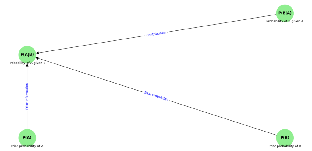
Bayes’ Theorem is one of the most important concepts in probability for data science. It helps you update the probability of an event happening based on new information. Think of it as a way to combine what you already know with new evidence to improve your prediction.
Here’s the formula for Bayes’ Theorem:

- P(A|B): The probability of event A happening, given that B is true (this is what we want to find).
- P(B|A): The probability of B happening, given that A is true.
- P(A): The overall probability of A happening (before any evidence is taken into account).
- P(B): The overall probability of B happening.
How to Use Bayes’ Theorem in Data Science
In data science, Bayes’ Theorem can help you make predictions when dealing with uncertain situations. For instance, if you’re trying to predict whether an email is spam or not, you can use Bayes’ Theorem to calculate the probability that an email is spam based on certain features, like the words used in the email.
Let’s say you have a set of emails, and you know the overall probability of an email being spam (P(A)). Then, if a new email contains the word “prize,” you can use Bayes’ Theorem to update the probability of the email being spam based on that word (P(B|A)).
Practical Applications of Bayes’ Theorem
One of the most common uses of Bayes’ Theorem in data science is in classification problems, especially in the Naive Bayes classifier. But it’s also used in various fields, such as medical diagnosis, finance, and machine learning, to update probabilities as new data comes in.
Naive Bayes Classifier
The Naive Bayes classifier is a machine learning algorithm that’s based on Bayes’ Theorem. It’s used for classifying data into different categories, especially when the features are independent of each other (hence the term “naive”).
Here’s how it works:
- You calculate the probability of each class given the features using Bayes’ Theorem.
- The algorithm assumes that each feature contributes independently to the final prediction, which simplifies the calculations.
Despite this “naive” assumption, the Naive Bayes classifier performs surprisingly well for tasks like spam detection, sentiment analysis, and document classification.
Example of Naive Bayes Classifier in Data Science with Bayes’ Theorem
Imagine you’re building an email spam filter. The classifier will predict whether an email is spam or not spam based on the words it contains. Let’s say the word “win” appears often in spam emails. Using Bayes’ Theorem, you can calculate the probability of an email being spam, given that it contains the word “win.”
Here’s a simplified way to explain it:
- P(Spam) = The overall probability of an email being spam (from all previous emails).
- P(Win|Spam) = The probability of seeing the word “win” in a spam email.
- P(Not Spam) = The probability of an email not being spam.
- P(Win|Not Spam) = The probability of seeing the word “win” in a non-spam email.
By plugging these probabilities into Bayes’ Theorem, you get a new probability that updates the chances of an email being spam based on the word “win.”
Why Naive Bayes Works So Well
The Naive Bayes classifier works particularly well when:
- You need speed: It’s computationally efficient and can handle large datasets quickly.
- Features are somewhat independent: While it assumes independence between features, it still works in many cases where that assumption doesn’t hold perfectly.
- You’re working with text: It’s widely used in natural language processing (NLP) tasks, such as spam detection and sentiment analysis, because text-based features (like word counts) often work well with this algorithm.
Real-World Applications of Probability in Data Science
Probability in Predictive Analytics
Predictive analytics is a fascinating area of data science that uses historical data to make predictions about future events. At the heart of predictive analytics lies probability. Understanding probability helps us build models that can forecast outcomes effectively.
How Probability Helps in Building Predictive Models
In predictive analytics, probability plays a crucial role in assessing the likelihood of various outcomes. Here’s how it works:
- Data Collection: First, relevant data is collected. This can include past sales figures, customer demographics, and seasonal trends.
- Modeling: Probability helps create models that can predict future events. For example, you might use logistic regression, which estimates the probability of an event occurring, such as whether a customer will buy a product based on their characteristics.
- Evaluation: Once the model is built, it’s essential to evaluate its performance. Metrics like accuracy, precision, and recall help assess how well the model predicts outcomes. These metrics rely on probability to determine the model’s reliability.
Example: Imagine you work for a retail company and want to predict which customers are likely to make a purchase. By analyzing historical purchase data, you can develop a model that assigns a probability score to each customer. If a customer has a 70% probability of making a purchase, marketing efforts can be targeted toward them, improving overall sales efficiency.
Here’s a simple representation of how this process looks:
| Step | Description |
|---|---|
| Data Collection | Gathering historical data about customer behavior |
| Modeling | Using algorithms to estimate probabilities of events |
| Evaluation | Assessing model accuracy and reliability |
Real-World Example: Probability in Predictive Analytics for Data Science
In healthcare, predictive analytics can help identify patients at risk of developing certain conditions. By analyzing patient data (like age, medical history, and lifestyle choices), healthcare providers can calculate the probability of a patient developing a condition like diabetes. This allows for early intervention and tailored care plans.
Probability and A/B Testing in Data Science
A/B testing is another significant application of probability in data science. This method compares two versions of a webpage or app to determine which one performs better.
How Probability Is Used to Analyze A/B Test Results
In A/B testing, probability helps analyze the results and make data-driven decisions. Here’s a breakdown of the process:
- Hypothesis Formation: You start with a hypothesis. For example, “Changing the color of the call-to-action button will increase click-through rates.”
- Random Assignment: Users are randomly assigned to two groups:
- Group A sees the original version (control).
- Group B sees the modified version (treatment).
- Data Collection: Data is collected on user interactions, such as clicks, conversions, or sign-ups.
- Statistical Analysis: Probability helps analyze the results. Statistical tests (like the t-test) determine if the differences between groups are statistically significant.
- Decision Making: Based on the analysis, decisions can be made. If the treatment group shows a significantly higher conversion rate, the new design may be implemented.
Example: Let’s say an online retailer wants to test two different layouts for their homepage. They might find that the new layout increases the conversion rate by 10%. Using statistical methods, they can calculate the probability that this improvement is due to the new design rather than random chance.
Here’s a simplified representation of the A/B testing process:
| Step | Description |
|---|---|
| Hypothesis Formation | Formulate a hypothesis about what will improve performance |
| Random Assignment | Split users into two groups randomly |
| Data Collection | Collect data on user behavior and outcomes |
| Statistical Analysis | Analyze results using probability and statistical tests |
| Decision Making | Decide which version to implement based on the analysis |
Using Probability for A/B Testing in Data Science
Using probability in A/B testing helps organizations make informed decisions. It reduces the guesswork involved in testing changes and allows for confident decision-making based on statistical evidence.
Latest Advancements in Probability for Data Science
Recent Research and Developments
The field of data science is always evolving, and the latest developments in probability theory are playing a significant role in enhancing artificial intelligence (AI) and machine learning (ML) models. Probability provides a mathematical framework that helps us quantify uncertainty and make predictions based on data. As we move further into the era of big data, these advancements are becoming even more crucial.
Importance of Probability in AI/ML Models
- Quantifying Uncertainty: In many real-world applications, data is noisy and incomplete. Probability helps in modeling this uncertainty, enabling better decision-making.
- Improved Predictions: By incorporating probability into models, predictions can be made more accurately. This is essential for applications like finance, healthcare, and marketing.
- Data-Driven Decisions: Advanced probability models provide insights that help organizations make informed choices. This is particularly valuable in competitive markets where every decision counts.
Bayesian Networks
One of the most exciting areas in the realm of probability for data science is the development of Bayesian networks. These graphical models represent a set of variables and their conditional dependencies using directed acyclic graphs.
The Role of Bayesian Networks in the Future of AI
Bayesian networks are making waves in AI and machine learning. They allow for the incorporation of prior knowledge and evidence into the modeling process, leading to improved predictions and decision-making.
- Structured Representation: Bayesian networks provide a structured way to represent complex relationships between variables. This is especially useful in domains like genetics, where multiple factors can influence outcomes.
- Real-Time Updates: With Bayesian networks, models can be updated in real time as new data becomes available. This dynamic updating process is vital in fast-paced environments like finance, where market conditions can change rapidly.
- Uncertainty Management: They excel at handling uncertainty. By using probabilities, these networks can assess the likelihood of various outcomes, making them invaluable for risk assessment and management.
Example: Imagine a healthcare scenario where a Bayesian network is used to predict the probability of a patient developing a certain disease based on symptoms and medical history. By analyzing the relationships between these variables, healthcare professionals can make informed decisions about diagnosis and treatment.
Here’s a simplified representation of how Bayesian networks work:
| Element | Description |
|---|---|
| Nodes | Represent variables (e.g., symptoms, diseases) |
| Edges | Indicate the relationships between variables |
| Conditional Probabilities | Quantify the strength of relationships and dependencies |
Advancements in Bayesian Networks
The advancements in Bayesian networks have made them more accessible and effective in various applications:
- Increased Computational Power: Modern algorithms and powerful computing resources have made it easier to work with complex Bayesian networks. This allows for handling larger datasets and more intricate models.
- Integration with Other Techniques: Bayesian networks can be combined with other machine learning techniques, such as neural networks. This integration enhances their predictive power and applicability.
- User-Friendly Tools: New software and tools have emerged that make building and analyzing Bayesian networks more user-friendly. This accessibility allows more data scientists and researchers to leverage these powerful models.
Conclusion: Mastering Probability for Data Science
As we wrap up our exploration of probability for data science, it’s essential to recap the key concepts we’ve discussed. Probability is not just a theoretical framework; it’s a practical tool that empowers data scientists to make informed decisions and build strong models. Here are the crucial points we’ve covered:
- Understanding Probability Distributions: We discussed various types of probability distributions, such as normal, binomial, and Poisson distributions. These distributions are foundational in analyzing data and making predictions.
- The Law of Large Numbers: This principle emphasizes that as the size of a sample increases, its mean will get closer to the expected value. This concept is vital for ensuring the reliability of your data analyses.
- Central Limit Theorem (CLT): We explored how the CLT states that the sampling distribution of the sample mean will be normally distributed, regardless of the original distribution, given a sufficiently large sample size. This theorem is crucial for hypothesis testing and creating confidence intervals.
- Bayes’ Theorem: This theorem allows us to update our beliefs based on new evidence, making it a powerful tool in decision-making and predictive modeling.
- Applications in Data Science: We highlighted the use of probability in predictive analytics, A/B testing, and the development of advanced models like Bayesian networks. These applications illustrate how probability helps analyze data and inform strategies across various fields.
Encouragement for Further Exploration
As you embark on your journey to mastering probability for data science success, I encourage you to explore more advanced concepts and apply these foundational ideas to real-world projects.
- Hands-On Practice: Engage with datasets, conduct experiments, and analyze the outcomes. Applying these concepts in practical scenarios will deepen your understanding.
- Further Learning: Consider diving into more advanced topics like stochastic processes, Markov chains, or machine learning algorithms that rely heavily on probability.
- Real-World Applications: Think about how you can use probability to solve problems in your field. Whether it’s predicting customer behavior, optimizing marketing strategies, or assessing risks in finance, the possibilities are endless.
Remember, mastering probability is a journey that opens doors to many opportunities in data science. Embrace the learning process, and don’t hesitate to experiment with different approaches. Your expertise in probability will be a powerful asset as you tackle more complex challenges in data science.
External Resources
StatQuest with Josh Starmer (YouTube Channel)
This YouTube channel breaks down complex statistics and probability concepts into easy-to-understand videos. It’s a great resource for visual learners who appreciate clear explanations and examples.
Visit StatQuest
Towards Data Science – Articles on Probability
Towards Data Science on Medium hosts numerous articles that discuss probability topics in data science, often with real-world examples and code snippets. A good way to see applications of probability in action.
Read on Towards Data Science
Wikipedia – Probability Theory
The Wikipedia page on probability theory provides a comprehensive overview of the concepts, history, and applications of probability, making it a good reference point for deeper research.
View Wikipedia
FAQs
What is probability in data science?
Probability in data science measures how likely an event is to occur. It helps data scientists make informed decisions based on the likelihood of various outcomes, guiding predictive models and analyses.
How is Bayes’ Theorem used in data science?
Bayes’ Theorem is used to update the probability of a hypothesis as more evidence becomes available. It’s fundamental in machine learning models like the Naive Bayes classifier, which predicts categories based on prior probabilities and observed features.
What are some common probability distributions used in data science?
Common probability distributions in data science include the Normal Distribution, which represents continuous data, the Binomial Distribution for binary outcomes, and the Poisson Distribution, which models the number of events in a fixed interval of time or space.
How does the Law of Large Numbers apply to data science?
The Law of Large Numbers states that as the sample size increases, the sample mean will get closer to the population mean. In data science, this principle ensures that larger datasets provide more accurate estimates and predictions, reducing the impact of random variations.







Leave a Reply