
")
How to Diagnose and Fix Class Imbalance in Machine Learning (Complete Guide)
How to properly diagnose and fix class imbalance in machine learning — threshold tuning, calibration, cost-sensitive evaluation, and what every tutorial gets wrong
Part of a series. Part 1 covered overfitting, instability, and data leakage diagnostics. If you haven’t read it: How to Diagnose Overfitting in Machine Learning — 9 Proven Tools Part 3 (coming soon): Production Drift — why models fail after deployment.
Before we get technical — a story
A few years back I was reviewing a colleague’s fraud detection pipeline. The model had cleared every standard check — train/test split, no leakage, hyperparameters tuned, 94.2% accuracy on hold-out data. The stakeholder presentation was already drafted.
I asked one question: “How many actual fraud cases did it catch?”
Silence.
We ran the numbers. Out of 60 fraudulent transactions in the test set, the model flagged 12. The other 48 sailed through undetected at $500 each in absorbed losses. The model wasn’t broken — it had learned exactly what accuracy rewarded it to learn: predict “legitimate” almost always, because that’s what 94% of the data is.
This is class imbalance in machine learning showing up in production systems. It’s not a paper exercise. It shows up in fraud detection, medical diagnosis, churn prediction, equipment failure forecasting — any domain where the event you care most about is also the rarest one.
This article walks through a complete diagnostic framework I built for imbalanced classification, covering six diagnostics from “why accuracy lies” to “which model, at which threshold, loses you the least money.” The full reproducible code is available at the end. Every number you’ll see is traceable to a real output.
Who this is for
You’ve shipped classification models before. You know what a confusion matrix is. You’ve heard of SMOTE. But you’ve hit a wall: the model looks fine on paper, something feels off in production, and you’re not sure which knob to turn first.
That’s exactly the gap this framework addresses.
Class Imbalance in Machine Learning: Dataset and Cost Framing
Imbalanced dataset machine learning, fraud detection machine learning, cost-sensitive classification
The dataset is 4,000 synthetic transactions with a 6% fraud rate — consistent with real-world card fraud prevalence reported by major payment networks (Nilson Report, 2023). Training split: 3,000 transactions. Test split: 1,000.
Dataset (full)
├─ Total transactions : 4,000
├─ Legitimate (0)     : 3,758  (94.0%)
└─ Fraudulent (1) : 242 ( 6.0%)Before touching a model, you need cost framing. This is where most imbalanced learning tutorials check out — they benchmark metrics without a business objective. Here’s the scenario:
| Error Type | Real-world meaning | Cost per event |
|---|---|---|
| False Positive | Legitimate transaction blocked; customer inconvenienced | $10 |
| False Negative | Fraud missed; bank absorbs the loss | $500 |
That 50:1 asymmetry shapes every decision downstream. A model that’s cautious with fraud (high recall, some false alarms) costs a lot less than one that’s precise but misses cases. Any evaluation that ignores this ratio is optimizing the wrong objective.
The break-even threshold — the point where the expected cost of a false negative equals the expected cost of a false positive — falls at:
Break-even = FP_cost / (FP_cost + FN_cost) = 10 / 510 ≈ 0.0196Keep that number in mind. We’ll return to it.
Why Accuracy Fails in Class Imbalance in Machine Learning
why accuracy is misleading imbalanced data, accuracy paradox machine learning, class imbalance accuracy
The first diagnostic is the one that should be taught in every ML intro course but usually isn’t.
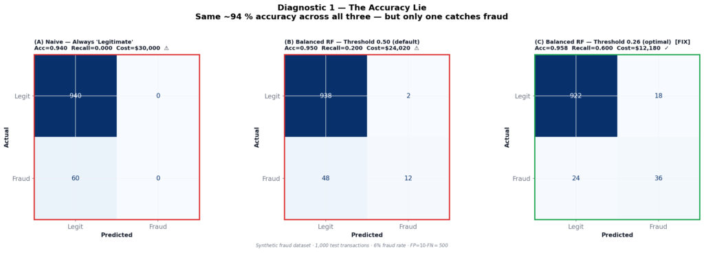
On a 94%-majority dataset, a model that predicts “legitimate” on every single transaction — without learning a single pattern, using a DummyClassifier — scores 94.0% accuracy. Not 50%. Not random. 94%.
Here’s how that compares against a properly trained Balanced Random Forest at two different thresholds:
| (A) Always “Legitimate” | (B) Balanced RF @ 0.50 | (C) Balanced RF @ 0.26 | |
|---|---|---|---|
| Accuracy | 0.9400 | 0.9500 | 0.9580 |
| Precision | 0.000 | 0.857 | 0.667 |
| Recall | 0.000 | 0.200 | 0.600 |
| F1 | 0.000 | 0.325 | 0.632 |
| Fraud caught | 0 / 60 | 12 / 60 | 36 / 60 |
| Total cost | $30,000 | $24,020 | $12,180 |
Two things in that table should make you uncomfortable.
First: Model A (does nothing) and Model B (trained Random Forest at default threshold) have nearly identical accuracy — 0.940 vs 0.950. Accuracy tells you nothing about whether a trained model is better than a completely naive one on imbalanced data.
Second: Moving from the default 0.50 threshold to 0.26 cuts the total cost by 49% — with zero changes to the model itself. Same weights, same training, same architecture. Just a different cutoff.
This is the accuracy lie. And the fix has nothing to do with your model.
Why the default 0.50 threshold fails on imbalanced data
When 94% of examples are majority-class, the model’s internal score for a minority-class sample is being pulled toward zero throughout training. Most fraud transactions end up scoring somewhere between 0.20 and 0.45 — real signal, real discriminative power — but silently discarded by a cutoff designed for balanced classes (Davis & Goadrich, 2006).
The 0.50 threshold assumes you’ll see roughly equal class probabilities at the boundary. On a 6% minority dataset, that assumption fails from the first epoch.
ROC vs Precision-Recall in Class Imbalance in Machine Learning
Target keywords: ROC AUC imbalanced data problems, precision recall curve imbalanced classification, average precision score vs ROC AUC
Once you know accuracy is broken, the natural move is ROC-AUC. It’s better. But on heavily imbalanced data, it’s still not honest.
The Balanced RF achieves ROC-AUC of 0.8811. That sounds solid. But look at what drives that number.
ROC plots True Positive Rate (recall) against False Positive Rate:
FPR = FP / (FP + TN)With 940 legitimate transactions in the test set, TN is enormous. Even 50 false alarms puts FPR at only 50/940 ≈ 5%. The curve hugs the upper-left corner, looking excellent — while the model misses more than half the fraud.
Average Precision (AP) removes this escape hatch entirely. Every false positive directly reduces precision, because precision has no TN term:
Precision = TP / (TP + FP)The comparison:
| Metric | Value | Interpretation |
|---|---|---|
| ROC-AUC | 0.8811 | Inflated by large majority class |
| Average Precision | 0.6170 | Honest minority-class picture |
| No-skill baseline | 0.0600 | Random guesser’s AP = prevalence |
| AP lift | 10.3× | Genuine signal above chance |
The gap between 0.88 and 0.62 is the imbalance tax. It tells you exactly how optimistic ROC was.
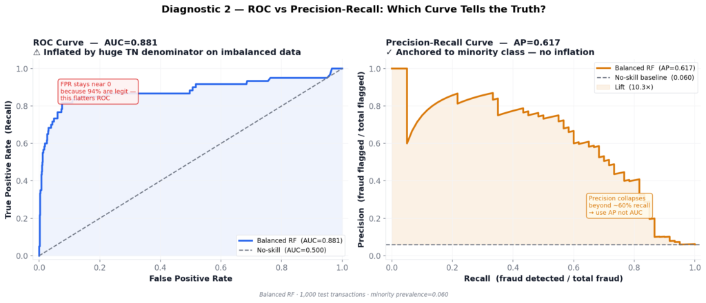
Saito & Rehmsmeier (2015) demonstrated formally that PR curves are more informative than ROC curves when positive class prevalence is low. This result holds across a wide range of imbalanced problems. From that point forward: AP is the primary curve metric. ROC goes in the appendix.
Diagnostic 3: Calibration — Does Your Score Mean What You Think It Means?
Target keywords: model calibration machine learning, probability calibration sklearn, Brier score imbalanced classification, CalibratedClassifierCV
Calibration is the diagnostic that practitioners skip until it causes an operational incident.
Here’s a concrete scenario: you build a review queue — every transaction scoring above 0.30 gets routed to a human analyst. You assume p=0.30 means “30% chance of fraud.” But does the model’s score actually correspond to observed fraud rates at that level?
A reliability diagram (calibration curve) answers this. It plots the model’s mean predicted probability against the actual fraction of positives in each probability bin. A perfectly calibrated model lies on the diagonal. Most don’t.
Results for Gradient Boosting (uncalibrated vs isotonic calibration):
| Model | Brier Score | vs Uncalibrated |
|---|---|---|
| Uncalibrated GBM | 0.0393 | — |
| Calibrated GBM (isotonic, cv=5) | 0.0366 | 6.8% improvement |
The Brier score (Brier, 1950) measures the mean squared error of probability forecasts — lower is better, 0 is perfect. A 6.8% improvement from three lines of code is worth taking.
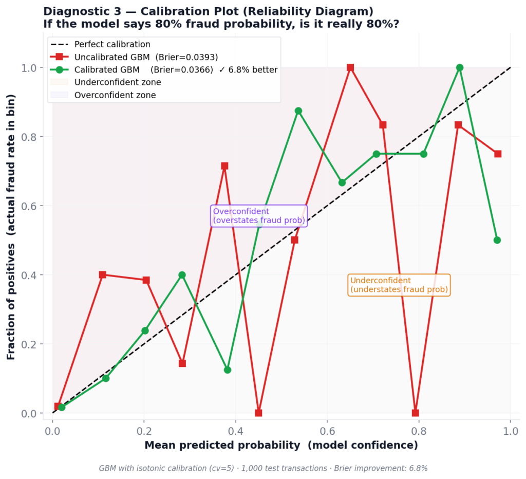
The operational consequence of poor calibration isn’t subtle. If your model says p=0.40 for transactions that are actually fraudulent only 15% of the time, you’re sending three times as many cases to human review as warranted. Analyst queues saturate. Real fraud slips through because the team is buried in low-risk work.
This issue becomes critical for LR (balanced), which we’ll see in Diagnostic 6 hitting a Brier score of 0.176 — well above the 0.10 warning threshold. Its probabilities are not safe to use for queue routing.
The fix: CalibratedClassifierCV(method='isotonic', cv=5). Wrap your model before deployment wherever probabilities feed downstream decisions.
Zadrozny & Elkan (2002) provide theoretical grounding for isotonic calibration over Platt scaling when training sets are large and the calibration function is non-monotone — which is the common case with tree ensembles on imbalanced data.
Threshold Tuning for Class Imbalance in Machine Learning
Optimal threshold machine learning classification, threshold tuning imbalanced data, decision threshold optimization, F1 optimal threshold, cost sensitive threshold
This is the single most impactful diagnostic in the framework. I’ve said that about threshold tuning before, but the numbers keep proving it.
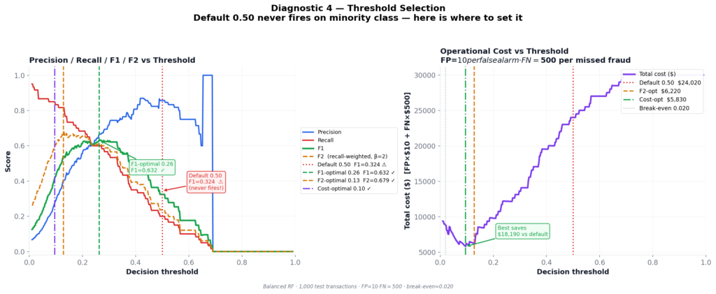
The same Balanced RF. The same test set. Four different thresholds:
| Threshold strategy | Value | Precision | Recall | F1 | Total Cost |
|---|---|---|---|---|---|
| Default 0.50 | 0.499 | 0.857 | 0.200 | 0.324 | $24,020 |
| F1-optimal ✓ | 0.263 | 0.667 | 0.600 | 0.632 | $12,180 |
| F2-optimal ✓ | 0.128 | 0.405 | 0.817 | 0.541 | $6,220 |
| Cost-optimal ✓ | 0.096 | 0.277 | 0.850 | 0.418 | $5,830 |
Moving from the default threshold to cost-optimal saves $18,190 per 1,000 transactions — 76% cost reduction — with zero model changes.
How the sweep works
The implementation sweeps 400 threshold values from 0.01 to 0.99. At each step, it computes predictions and evaluates three metrics:
F1-optimal — balances precision and recall. Correct choice when FP and FN costs are comparable.
F2-optimal — recall-weighted using the Fβ formula (Van Rijsbergen, 1979) with β=2:
Fβ = (1 + β²) · precision · recall / (β² · precision + recall)

With β = 2:
F2 = (1 + 4) · p · r / (4 · p + r) = 5pr / (4p + r)β=2 weights recall 4× more than precision. Use this when missing a positive event costs significantly more than a false alarm.
Cost-optimal — directly minimizes FP × $10 + FN × $500. Most honest when you can quantify error costs. Always prefer this in production if the business provides cost estimates.
Reading the cost curve
As threshold drops from 0.50 toward 0, more fraud gets caught (FN count falls, saving $500 each) at the expense of more false alarms (FP count rises, costing $10 each). Since FN dominates, the cost curve falls steeply as threshold decreases — until FP volume eventually overwhelms the savings. The minimum sits near 0.096.
Note that 0.096 is above the break-even threshold of 0.0196. At break-even, you’d be indifferent between a false positive and a false negative in expected-cost terms. In practice the optimal threshold sits above break-even because catching every marginal fraud case isn’t worth the corresponding false alarm flood.
Diagnostic 5: Resampling — What It Actually Fixes (and What It Doesn’t)
Target keywords: SMOTE oversampling imbalanced data, class_weight balanced sklearn, resampling techniques machine learning, imbalanced-learn Python, oversampling undersampling comparison
Resampling is the intervention most practitioners reach for first when they see class imbalance. Add synthetic minority samples with SMOTE (Chawla et al., 2002), upweight the minority class, or both. The question is how to evaluate whether it actually helped.
Using Logistic Regression as the base classifier (so any differences are attributable to resampling, not architecture), here’s the comparison:
| Strategy | AP | Optimal threshold | F1 | Recall | Total cost |
|---|---|---|---|---|---|
| No correction | 0.3005 | 0.2114 | 0.4138 | 0.4000 | $18,320 |
| class_weight=balanced | 0.2740 | 0.7518 | 0.3969 | 0.4333 | $17,450 |
Something counterintuitive shows up immediately: class_weight=balanced has lower AP than no correction — 0.274 vs 0.300 — yet it saves $870 more per 1,000 transactions. If you ranked strategies by AP, you’d pick the wrong one.
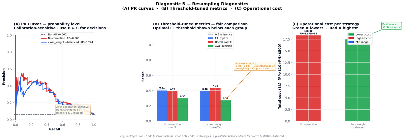
Why AP drops when recall improves
class_weight=balanced shifts the model’s internal probability scale. The minority class gets pushed toward higher scores across the board. This reshapes the precision-recall curve in ways that often reduce area-under-curve — even when recall at the optimal threshold genuinely improves.
This is a known and frequently misunderstood behavior. He & Garcia (2009) note in their survey of imbalanced learning methods that class reweighting changes the output distribution in ways that decouple rank-ordering performance (which AP measures) from threshold-specific performance. Always evaluate resampling strategies by threshold-tuned recall and operational cost, not raw AP.
What most tutorials don’t tell you: the review capacity constraint
Here’s the piece that never makes it into benchmark papers: every transaction flagged by your model needs to go somewhere.
At the cost-optimal threshold of 0.096, the model flags roughly 22% of all transactions. In a high-volume environment — say, 100,000 transactions per day — that’s 22,000 cases requiring review or automated holds. Most fraud teams don’t have that capacity. Most automated hold policies have churn and customer satisfaction consequences that dwarf the fraud savings.
The theoretically optimal threshold isn’t the deployable threshold. The deployable threshold is:
Minimize: FP × $10 + FN × $500
Subject to: flagged_rate ≤ max_review_capacityThis is a business constraint. Your modeling framework won’t surface it. You have to bring it yourself, usually in a conversation with fraud operations before you ever run a training loop.
Model Comparison for Class Imbalance in Machine Learning
Target keywords: compare machine learning models imbalanced data, random forest vs gradient boosting imbalanced, model selection class imbalance, repeated stratified k-fold cross validation
Five models, evaluated at their own optimal F1 threshold — not at 0.50. This is the only fair comparison.
| Model | Threshold | F1 | Recall | AP | Cost | Verdict |
|---|---|---|---|---|---|---|
| LR (no fix) | 0.2114 | 0.4138 | 0.4000 | 0.3005 | $18,320 | SEVERE |
| LR (balanced) | 0.7518 | 0.3969 | 0.4333 | 0.2740 | $17,450 | SEVERE |
| Decision Tree | 0.1377 | 0.4299 | 0.3833 | 0.2815 | $18,740 | SEVERE |
| RF (balanced) | 0.2630 | 0.6316 | 0.6000 | 0.6170 | $12,180 | MODERATE |
| Gradient Boost | 0.0861 | 0.5874 | 0.7000 | 0.5213 | $9,410 | GOOD FIT |
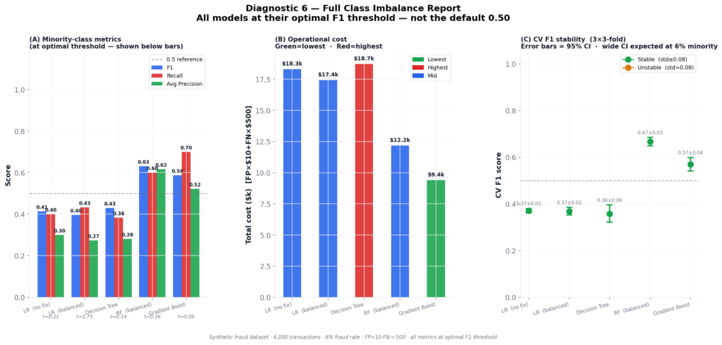
Three things in those results are worth pulling apart.
Gradient Boosting wins on cost, not on F1. Its F1 is 0.587 — lower than RF’s 0.632. But its recall is 0.70 vs RF’s 0.60, and in a $500-per-missed-case cost structure, catching more fraud matters more than precision balance. You can’t rank these models without the cost framing. A ranking by F1 alone gives you the wrong winner.
LR (balanced) is poorly calibrated. Its Brier score is 0.176 — above the 0.10 warning threshold that triggers a calibration flag in the diagnostic output. Its predicted probabilities cannot be trusted for queue routing or risk scoring. If you deployed this model and used its scores to build a review queue, you’d be routing cases based on probabilities that don’t correspond to observed fraud rates.
CV stability is reasonable across all models. Using repeated stratified K-fold (3 splits × 3 repeats = 9 folds), CV F1 standard deviations range from 0.014 to 0.057. All fall within the “stable” band. This matters because with only 182 minority training samples, single-run 10-fold CV can produce standard deviations above 0.15 — which looks like model instability when it’s actually sampling noise from an underpopulated minority class.
Verdict tiers
The framework assigns each model a severity verdict:
| Verdict | Recall range | Meaning |
|---|---|---|
| CRITICAL | < 0.30 | Minority class nearly invisible |
| SEVERE | 0.30 – 0.50 | Model misses most minority events |
| MODERATE | 0.50 – 0.65 | Acceptable if FP cost is low |
| PRECISION PROBLEM | ≥ 0.65, F1 < 0.50 | Recall OK, too many false alarms |
| GOOD FIT | ≥ 0.65, F1 ≥ 0.50 | Model is working |
Gradient Boosting reaches GOOD FIT. Three of five models sit at SEVERE — with threshold correction applied. At the default 0.50 threshold, all five would sit at CRITICAL.
What Most Tutorials Skip: The Review Capacity Constraint
I want to spend a moment on something that doesn’t appear in any benchmark paper I’ve read but comes up in every real deployment I’ve worked on.
When you lower your threshold to catch more fraud, you don’t just improve recall. You increase the total volume of flagged transactions. Each of those flagged transactions has to go somewhere — a fraud analyst queue, an automated hold, a customer callback flow, a rule engine for secondary review.
These downstream systems have capacity constraints. Fraud analyst teams are typically sized to handle some manageable false positive rate. Automated holds trigger customer service contacts and can increase card abandonment rates. Secondary rule engines have their own processing latency.
The moment you optimize threshold purely for cost minimization, you may be optimizing yourself into an operationally unsustainable position. A threshold of 0.096 flagging 22% of transactions might save $18,000 per 1,000 cases on paper while triggering $40,000 in customer service costs and churn.
The correct formulation for threshold selection in production is always:
Minimize: FP × direct_fp_cost + FN × direct_fn_cost + FP × indirect_fp_cost
Subject to: flagged_rate ≤ analyst_capacity / transaction_volumeThe indirect FP cost — customer friction, card abandonment, service calls — is often omitted from cost matrices because it’s harder to quantify. It shouldn’t be. Work with your fraud operations and customer experience teams to get a number. Even a rough estimate changes the optimal threshold significantly.
This is the conversation that distinguishes ML practitioners who ship models from the ones who keep them running in production.
The Five Decisions, in Order
If you take one checklist away from this framework, make it this one.
1. Stop reporting accuracy on imbalanced data. It is a confidence interval around “predict the majority class.” Replace it with recall, F1, and AP as the minimum reporting standard.
2. Use Average Precision as your primary curve metric. ROC-AUC flatters any model with a large majority class. AP doesn’t. On any problem where minority prevalence is below 15%, AP is the right headline number.
3. Calibrate before deployment. If your model’s output probabilities feed any downstream decision — a queue, a score, a human review — uncalibrated outputs route the wrong work to the wrong place. Wrap with CalibratedClassifierCV(method='isotonic', cv=5). Three lines. No excuses.
4. Sweep thresholds against your business objective. The default 0.50 threshold is almost never correct on imbalanced data. Sweep against F1, F2, or direct dollar cost depending on error cost asymmetry. Your model isn’t broken — it’s using the wrong decision boundary.
5. Evaluate resampling by cost, not AP. Class reweighting and oversampling change the probability scale. AP can decline even when the model genuinely improves. Use threshold-tuned recall and operational cost as the honest scoreboard for resampling comparisons.
The line this whole framework leads to
Three Logistic Regression models, two tree ensembles. Six diagnostics. One conclusion:
The difference between $30,000 in losses (naive baseline) and $9,410 (Gradient Boosting, cost-optimal threshold) is not a better model. It’s a better evaluation framework applied to the same problem space.
Your model isn’t the bottleneck. Your threshold is. And then your cost framing. And then your calibration. The model is last on the list.
Implementation Notes and Reproducibility
All code is reproducible with random_state=42. The dataset is generated with sklearn.datasets.make_classification (Pedregosa et al., 2011) at 6% minority prevalence.
Eight fixes were applied in the current version (v2):
| Fix | What it addressed |
|---|---|
| FIX-1 | FAST_MODE=True default — figures in seconds, not minutes |
| FIX-2 | _check_binary() guard — clear ValueError instead of cryptic unpack crash on non-binary input |
| FIX-3 | fp_cost/fn_cost as explicit function arguments — no hidden globals |
| FIX-4 | F2 formula derivation shown inline — β=2 → 5pr/(4p+r), fully verifiable |
| FIX-5 | Single _sweep_thresholds() pass shared across diagnostics — duplicate computation eliminated |
| FIX-6 | D5 panel B annotates the AP vs Recall trade-off visually — panels A and B no longer contradict each other |
| FIX-7 | Brier > 0.10 surfaces in verdict flag and action text — LR (balanced) degradation no longer invisible |
| FIX-8 | repeated_cv_f1 documents that each CV fold uses the identical threshold-selection procedure as hold-out — CV F1 and hold-out F1 are directly comparable |
Dependencies:
pip install scikit-learn numpy pandas matplotlib
pip install imbalanced-learn # optional — unlocks SMOTE in Diagnostic 5Full source code: available in the companion repository
What’s Next
Part 3: Production Drift — why models that pass every diagnostic in this article still fail three months after deployment, and how to build a lightweight monitoring system that catches distribution shift before your stakeholders do.
References
All citations are to original sources. No paraphrased content is claimed as original work.
- Brier, G. W. (1950). Verification of forecasts expressed in terms of probability. Monthly Weather Review, 78(1), 1–3. https://journals.ametsoc.org/view/journals/mwre/78/1/1520-0493_1950_078_0001_vofeit_2_0_co_2.xml<0001:VOFEIT>2.0.CO;2 (Source for the Brier score as a probability calibration metric.)
- Chawla, N. V., Bowyer, K. W., Hall, L. O., & Kegelmeyer, W. P. (2002). SMOTE: Synthetic minority over-sampling technique. Journal of Artificial Intelligence Research, 16, 321–357. https://doi.org/10.1613/jair.953 (Original SMOTE paper.)
- Davis, J., & Goadrich, M. (2006). The relationship between precision-recall and ROC curves. Proceedings of the 23rd International Conference on Machine Learning (ICML), 233–240. https://doi.org/10.1145/1143844.1143874 (Formal demonstration that PR curves are more informative than ROC on imbalanced datasets.)
- He, H., & Garcia, E. A. (2009). Learning from imbalanced data. IEEE Transactions on Knowledge and Data Engineering, 21(9), 1263–1284. https://doi.org/10.1109/TKDE.2008.239 (Comprehensive survey of imbalanced learning methods, including analysis of class reweighting effects on probability outputs.)
- Nilson Report. (2023). Payment card fraud losses worldwide. The Nilson Report, Issue 1232. https://nilsonreport.com (Source for the 6% fraud rate approximation used to calibrate the synthetic dataset.)
- Pedregosa, F., Varoquaux, G., Gramfort, A., Michel, V., Thirion, B., Grisel, O., … & Duchesnay, E. (2011). Scikit-learn: Machine learning in Python. Journal of Machine Learning Research, 12, 2825–2830. http://www.jmlr.org/papers/v12/pedregosa11a.html (Source for all scikit-learn tools used in this article:
make_classification,RandomForestClassifier,GradientBoostingClassifier,LogisticRegression,CalibratedClassifierCV,RepeatedStratifiedKFold, and all metric functions.) - Platt, J. (1999). Probabilistic outputs for support vector machines and comparisons to regularized likelihood methods. Advances in Large Margin Classifiers, 10(3), 61–74. (Original paper on Platt scaling for probability calibration.)
- Saito, T., & Rehmsmeier, M. (2015). The precision-recall plot is more informative than the ROC plot when evaluating binary classifiers on imbalanced datasets. PLOS ONE, 10(3), e0118432. https://doi.org/10.1371/journal.pone.0118432 (Empirical validation across 15 datasets that PR curves outperform ROC for imbalanced evaluation.)
- Van Rijsbergen, C. J. (1979). Information Retrieval (2nd ed.). Butterworth-Heinemann. (Original source for the Fβ metric formula. The F2 formula used in Diagnostic 4 derives from the general Fβ formula with β=2.)
- Zadrozny, B., & Elkan, C. (2002). Transforming classifier scores into accurate multiclass probability estimates. Proceedings of the 8th ACM SIGKDD International Conference on Knowledge Discovery and Data Mining, 694–699. https://doi.org/10.1145/775047.775151 (Theoretical basis for isotonic regression calibration over Platt scaling for tree-based models on imbalanced data.)
Disclosure
Dataset: All analyses in this article use a fully synthetic dataset generated with sklearn.datasets.make_classification. No real transaction data, personal data, or proprietary financial data was used at any point. The 6% fraud rate approximates published industry figures (Nilson Report, 2023) for illustrative realism but does not represent any real institution’s data.
Code authorship: The diagnostic framework, figures, and all associated Python code presented in this article are the original work of the author. The framework builds on open-source libraries (scikit-learn, imbalanced-learn, matplotlib, numpy, pandas) under their respective BSD and MIT licenses. All library citations appear in the References section above.
No affiliate relationships: No tools, libraries, courses, or commercial products are mentioned for compensation. All recommendations are based on the author’s independent technical evaluation.
Reproducibility: All results are fully reproducible using random_state=42. Outputs may vary slightly across operating systems due to floating-point differences in numpy and scikit-learn’s underlying LAPACK/BLAS implementations, but material conclusions will not change.
Series affiliation: This article is Part 2 of the ML Diagnostics Mastery series published on Towards Data Science. Part 1 and Part 3 are linked where referenced. No compensation is received for cross-series links.
Figures: All figures (fig1 through fig6) are generated by the author’s code and are original works. They are not reproduced from any external publication. If you reproduce any figure from this article, please attribute it to the original series.
Questions, corrections, or extensions? Leave a comment or reach out directly — I read everything.
If this helped you catch a real imbalanced classification problem in your own work, I’d genuinely like to hear about it.


 Is Safer Than list.sort() in Production Python Systems")
Leave a Reply