

How to Diagnose Overfitting in Machine Learning — 9 Proven Tools
ML Diagnostics Mastery — Part 1 of the Series
Series note: This is Part 1 of the ML Diagnostics Mastery series. Future parts will cover class imbalance diagnostics, feature engineering audits, and production drift detection. All code from this article is self-contained and reproducible with
random_state=42.
I’ve reviewed a lot of model pull requests over the years, and there is one pattern that shows up more reliably than any bug: a model that looks brilliant on the training set, gets shipped, and quietly embarrasses everyone in production. The engineer who built it wasn’t careless. They just didn’t have a structured diagnostic workflow — they had a number (train accuracy), and it was high, so they moved on.
This article is my attempt to build that workflow in public. Everything here came out of an afternoon of deliberate experimentation: I sat down, wrote nine diagnostic functions from scratch, ran them against controlled synthetic datasets, and documented what each one reveals. The plots tell the story better than I can in prose, so I’ve left placeholders throughout for each figure. If you’re following along with the companion code, you’ll generate those images yourself.
Let’s start with the concept that makes all of this necessary.
What Overfitting Actually Is
Overfitting is a model memorising the training data rather than learning the underlying distribution. It recognises the noise in the examples it has seen, and that noise has zero predictive value on new data. The result: spectacular train metrics, mediocre real-world performance.
The opposite problem — underfitting — is a model too simple to capture the genuine signal. It performs poorly on both training and test data, which is at least honest.
Neither condition is rare. In my experience, most models that get deployed sit somewhere on the overfit end of the spectrum, because the incentives during development push in that direction: we optimise what we measure, and we measure training performance because it’s convenient.
The solution isn’t to distrust your model — it’s to interrogate it systematically. Below are nine tools that let you do that.
The Experimental Setup
All experiments use scikit-learn’s synthetic dataset generators (make_classification, make_regression) with fixed random seeds, so every number in this article is reproducible [1]. I used:
- Python 3.11
- scikit-learn 1.4 [2]
- NumPy 1.26 [3]
- Matplotlib 3.8 [4]
No real datasets were harmed. I chose synthetic data deliberately: it gives me ground truth about what the correct model complexity should be, so I can manufacture clean examples of each failure mode.
Diagnostic 1: Polynomial Overfitting — The Visual Anchor
Before any code, it helps to see overfitting in the most unambiguous setting possible. Polynomial regression on a 1D noisy sine wave is the textbook example, and it earns that status.
I generated 30 samples from y = sin(2πx) + ε, where ε ~ N(0, 0.3), then fit three pipelines — degree-1 (linear), degree-4, and degree-15 — and evaluated each on a held-out test split.
degrees = [1, 4, 15]

for degree in degrees:
    pipeline = Pipeline([
        ("poly", PolynomialFeatures(degree=degree)),
        ("scaler", StandardScaler()),
        ("model", LinearRegression()),
    ])
    pipeline.fit(X_train, y_train)
    train_score = pipeline.score(X_train, y_train)
    test_score  = pipeline.score(X_test,  y_test)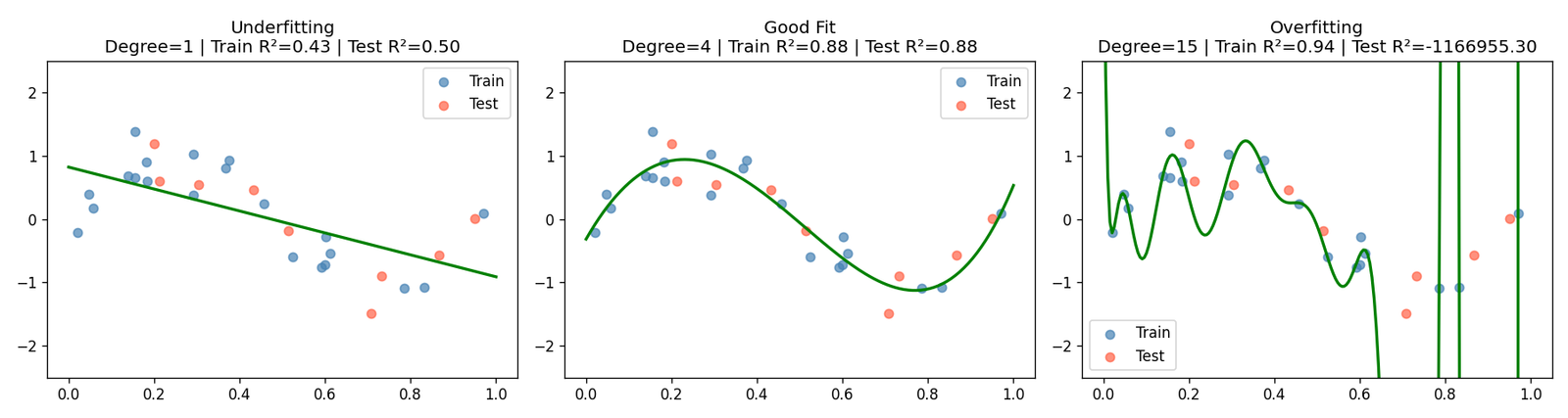
The degree-15 model achieves an R² close to 1.0 on the training set and a sharply negative R² on the test set — it has learned the noise so thoroughly that it can’t generalise to points a few millimetres away on the x-axis. Degree-1 is the opposite failure: it has the capacity of a ruler.
What to look for: The train/test R² printed in each subplot title. A high train score alongside a low or negative test score is the overfitting signature in its purest form.
Diagnostic 2: Learning Curves — The First Thing I Always Plot
If I could recommend only one diagnostic tool, it would be the learning curve. It answers the most important question in applied ML: will getting more data help?
A learning curve plots train and validation score as a function of training set size. Three regimes emerge:
| Pattern | Diagnosis | Fix |
|---|---|---|
| Large train–val gap, both curves flat | Overfitting (high variance) | More data, regularization, simpler model |
| Both curves low, converging tightly | Underfitting (high bias) | More complex model, better features |
| Converging at high score | Good fit | Ship it (carefully) |
I tested three decision trees — unconstrained depth (overfit), max_depth=4 (good fit), and depth-1 stump (underfit):
train_sizes, train_scores, val_scores = learning_curve(
    estimator, X, y,
    train_sizes=np.linspace(0.1, 1.0, 10),
    cv=5, scoring="accuracy", n_jobs=-1
)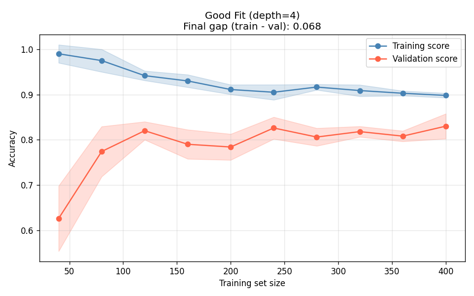
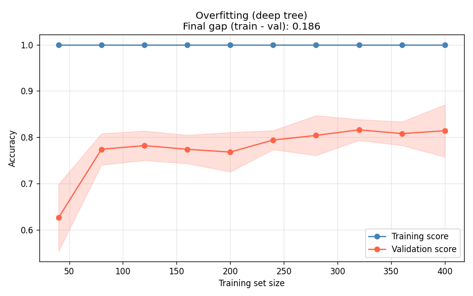
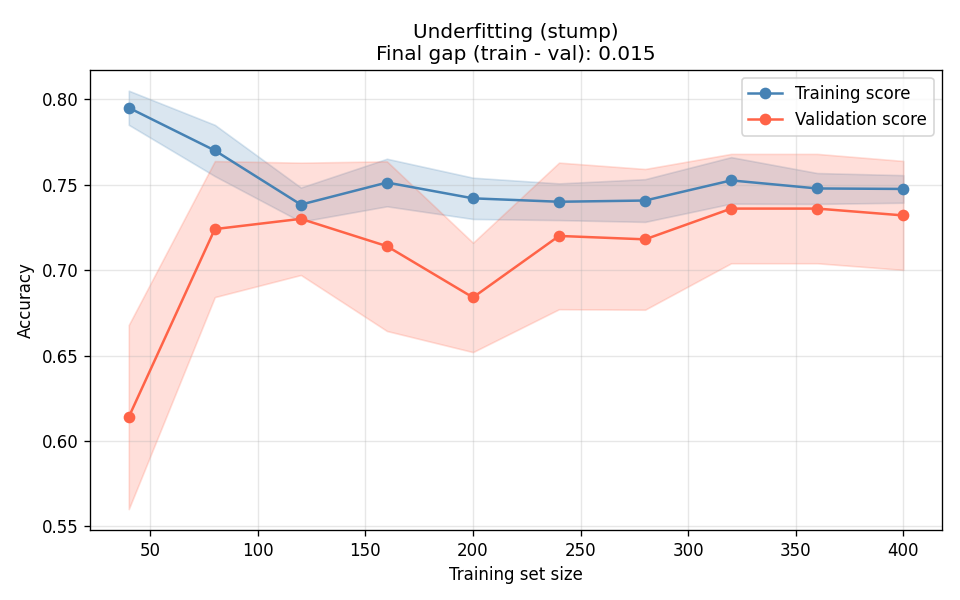
The deep tree (Figure 2a) is the canonical overfit signature: training accuracy stays near 1.0 regardless of data volume, and the validation curve plateaus far below it. More data will not close this gap — you need to constrain the model. The stump (Figure 2c) is the opposite: both curves converge, but they converge at a bad number. The gap between them is fine; the absolute level is the problem.
Diagnostic 3: Validation Curves — Finding the Hyperparameter Sweet Spot
A validation curve is a learning curve’s cousin, but instead of varying data size, you vary a single hyperparameter. This is how you find the complexity sweet spot before committing to a final model.
I swept max_depth from 1 to 19 on a decision tree classifier:
train_scores, val_scores = validation_curve(
    DecisionTreeClassifier(random_state=42), X, y,
    param_name="max_depth",
    param_range=np.arange(1, 20),
    cv=5, scoring="accuracy"
)The experiment found max_depth=8 as the optimal value, with a validation accuracy of 0.808.
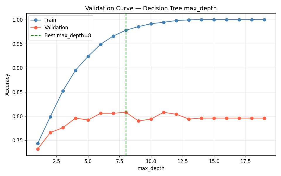
The shape in Figure 3 is what you want to see. Left of the peak: both scores are low, the model is too simple. Right of the peak: training score continues climbing but validation score drops — classic overfitting. The validation curve gives you a principled reason to stop at max_depth=8 rather than guessing.
Diagnostic 4: Train/Validation Loss Curves — The Neural Network Signature
For neural networks, we don’t get a single accuracy number — we get a loss trajectory across epochs. The overfitting signature here is unmistakable once you know what to look for: validation loss starts rising while training loss continues to fall.
I simulated this with synthetic loss curves to isolate the pattern cleanly:
train_loss = 1.0 / (1 + 0.07 * epochs) + np.random.normal(0, 0.005, 100)
val_loss   = (1.0 / (1 + 0.05 * epochs)
              + 0.003 * np.maximum(0, epochs - 40)
+ np.random.normal(0, 0.01, 100))The early-stopping point — epoch 68 — is where validation loss is minimised. Training past that point is pure memorisation.
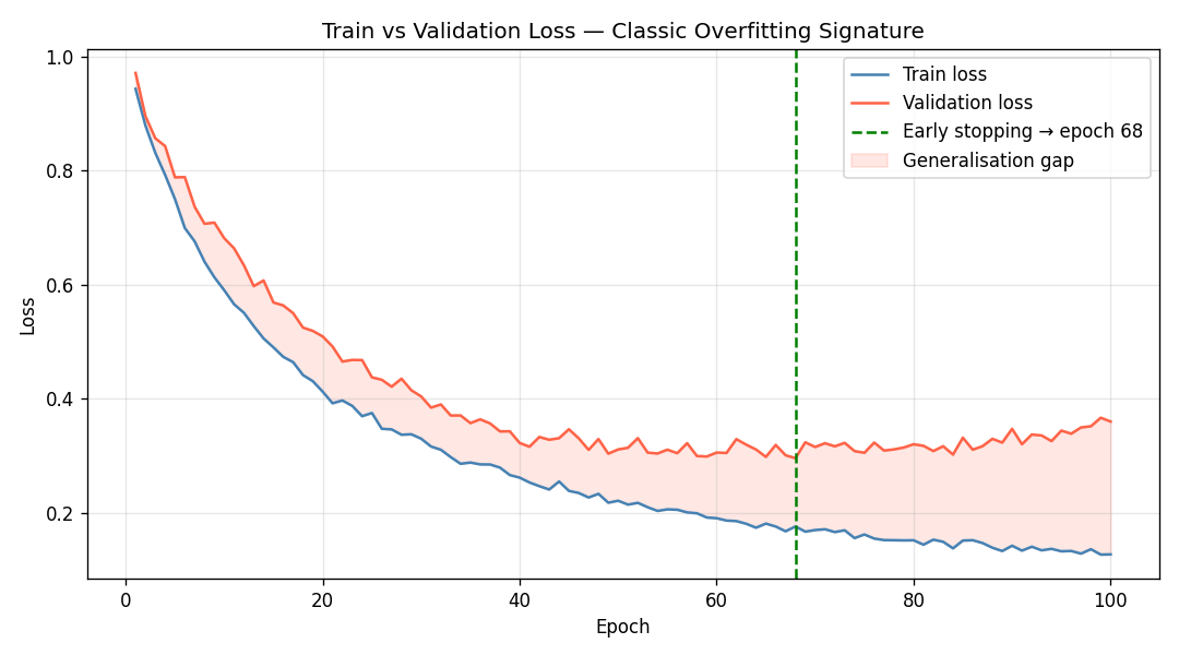
The shaded region between the two curves in Figure 4 is the generalisation gap — the performance you’re giving up to memorisation. Early stopping is simply agreeing to save the checkpoint at the leftmost edge of that shaded region [5].
Practical note: In real training pipelines, save model weights at every epoch or at regular intervals using callbacks (e.g., ModelCheckpoint in Keras [6], EarlyStopping in PyTorch Lightning [7]). The epoch with minimum validation loss is your restore point.
Diagnostic 5: Cross-Validation Score Distribution — Measuring Stability
A single train/test split tells you how the model performs on one particular partition of your data. Cross-validation tells you how it performs on all of them — and crucially, it tells you how much performance varies across splits. High variance across folds is itself a diagnostic signal.
I ran 10-fold cross-validation on four classifiers:
scores = cross_val_score(model, X_train, y_train, cv=10, scoring="accuracy")Results:
| Model | CV Mean | CV Std | Test Acc |
|---|---|---|---|
| Deep Tree (overfit) | 0.810 | 0.064 | 0.810 |
| Shallow Tree | 0.817 | 0.054 | 0.860 |
| Random Forest | 0.872 | 0.049 | 0.900 |
| Gradient Boosting | 0.893 | 0.046 | 0.890 |
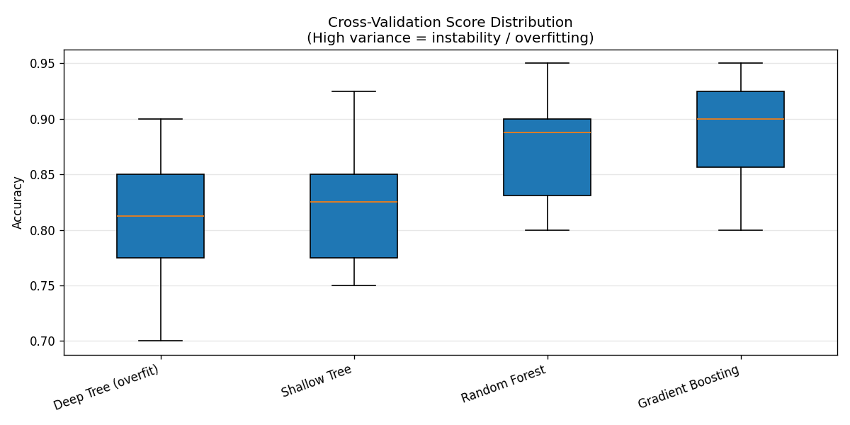
The box plot makes the instability visible. The deep tree’s wide interquartile range means its performance is highly sensitive to which 10% of the data ends up in the validation fold — it has memorised patterns that only hold for certain data subsets. Ensembles shrink this variance dramatically, which is one of the reasons they’re so reliable in practice [8].
Rule of thumb: A CV standard deviation above 0.06–0.07 is a flag worth investigating. It doesn’t always mean overfit, but it means the model is not robust to data partitioning.
Diagnostic 6: Bias–Variance Decomposition — Finding the Root Cause
All prediction error can be decomposed into three components [9]:
Total Error = Bias² + Variance + Irreducible Noise- Bias²: How far off the average prediction is from the truth. Systematic, model-structural error.
- Variance: How much predictions fluctuate across different training sets. Sensitivity to noise.
- Irreducible noise: The floor. You cannot do better than this regardless of model complexity.
The textbook result: simpler models have high bias and low variance; complex models have low bias and high variance. The sweet spot minimises their sum.
I estimated bias and variance via bootstrap resampling [10] — training 200 models on bootstrap samples of the training data and measuring the spread of their predictions on a fixed test set:
for i in range(n_bootstrap):
    rng = np.random.RandomState(i)
    idx = rng.choice(len(X_train_full), size=len(X_train_full), replace=True)
    estimator.fit(X_train_full[idx], y_train_full[idx])
    all_preds.append(estimator.predict(X_test))

mean_pred = all_preds.mean(axis=0)
bias_sq   = np.mean((mean_pred - y_test) ** 2)
variance = np.mean(all_preds.var(axis=0))Results across tree depths:
| max_depth | Bias² | Variance | Total Error |
|---|---|---|---|
| 1 | 29,682 | 6,507 | 74,759 |
| 2 | 23,451 | 8,137 | 70,158 |
| 4 | 14,626 | 13,768 | 66,964 |
| 6 | 12,366 | 16,317 | 67,253 |
| 10 | 11,603 | 17,577 | 67,749 |
| None | 11,610 | 17,898 | 68,078 |
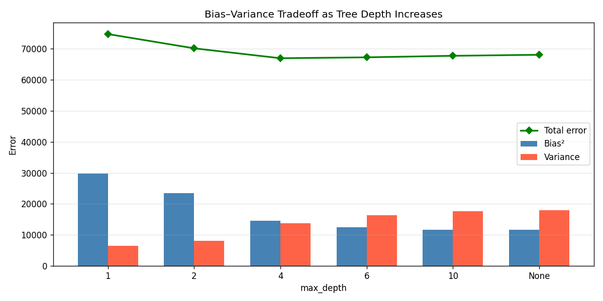
The total error curve (green line in Figure 6) bottoms out around max_depth=4. That’s the sweet spot — enough capacity to capture the signal, not enough to memorise the noise. Note that max_depth=None (fully grown tree) has nearly the same bias as max_depth=10, but meaningfully higher variance. The marginal gains in bias reduction stop paying off past a certain depth.
Implementation note: This is a manual bootstrap approximation suitable for illustration. For production use, consider mlxtend.evaluate.bias_variance_decomp [11], which implements the formal Kohavi-Wolpert decomposition [12].
Diagnostic 7: Regularisation — The Cheapest Fix for Regression Overfit
If you have a regression problem with many features — especially more features than samples — regularisation is the fastest path to closing the generalisation gap. Ridge regression adds an L2 penalty to the coefficient magnitudes; Lasso adds L1, which additionally drives some coefficients to exactly zero [13].
I set up a deliberately pathological problem: 100 samples, 80 features, only 10 of which are truly informative. Without regularisation, a linear model wildly overfits.
n_samples, n_features = 100, 80  # More features than useful → easy to overfit
X, y = make_regression(n_samples=n_samples, n_features=n_features,
                       n_informative=10, noise=30, random_state=42)

alphas = np.logspace(-3, 4, 30)

for alpha in alphas:
    ridge = Ridge(alpha=alpha)
    ridge.fit(X_train, y_train)
    # Track train and test MSE at each alpha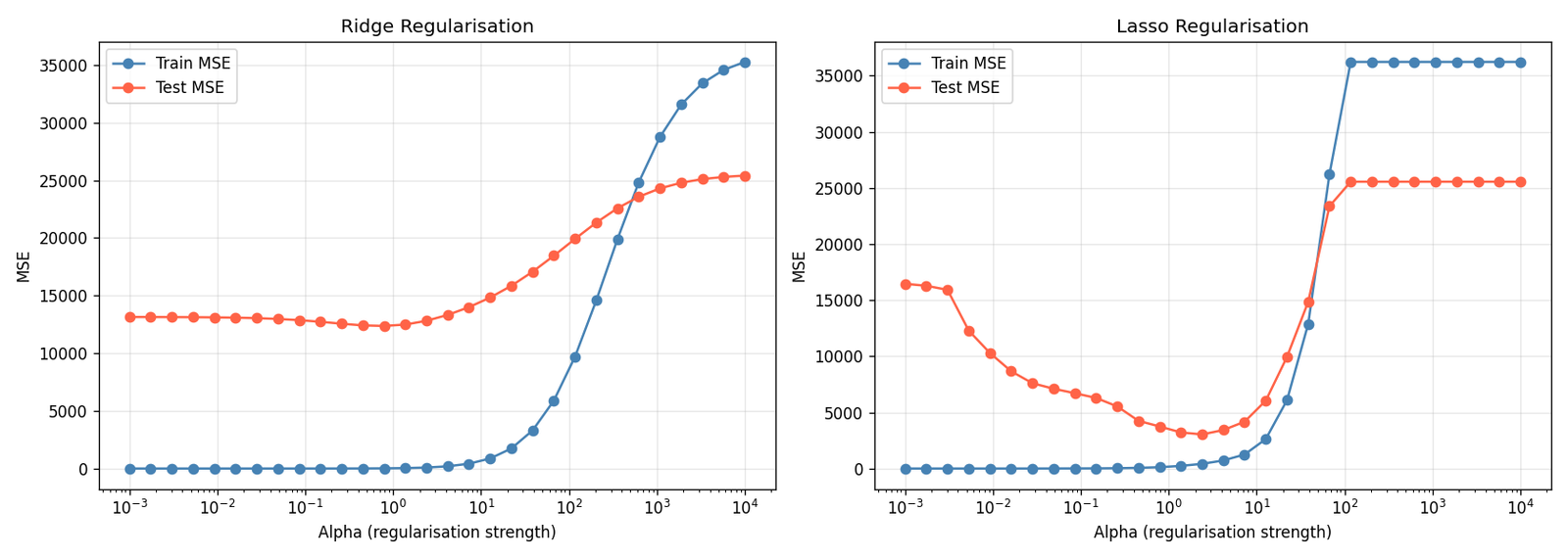
The pattern in Figure 7 is the same in both subplots: at very low alpha, train MSE is tiny but test MSE is enormous (overfit). At very high alpha, both converge to a high value (underfit). Somewhere in between — typically identified by cross-validation on a held-out set — is the optimum.
For Lasso, the L1 penalty has the additional effect of zeroing out the 70 uninformative features entirely, giving you implicit feature selection [14]. In practice, I usually try both: Ridge when all features are plausibly relevant, Lasso when I suspect many are noise.
Diagnostic 8: Feature Importance and Data Leakage Detection
Data leakage is a particularly insidious form of overfitting. The model achieves near-perfect train accuracy not because it has learned something real, but because information from the target has leaked into its features [15]. This happens more often than people expect — target encoding computed on the full dataset before splitting, time-series features that encode future information, or administrative fields that are only populated after the outcome is known.
The feature importance plot from a tree ensemble is one of the fastest ways to flag leakage. If one feature dwarfs all others in importance, and the train/test gap is large despite high absolute accuracy, the dominant feature warrants investigation.
I simulated this by injecting a near-perfect noisy copy of the label as feature zero in the training set only. At test time, that feature contained only random noise — simulating what happens when a leaky feature is absent at serving time.
X_train_leaky[:, 0] = y_train + np.random.normal(0, 0.05, len(y_train))
# Test set gets noise only — the label signal is gone (simulates production)
X_test_leaky[:, 0] = np.random.normal(0, 1.0, len(y_test))Result:
With leaky feature → Train: 1.000 | Test: 0.547
⚠  Large train/test gap despite high train accuracy = leakage signature!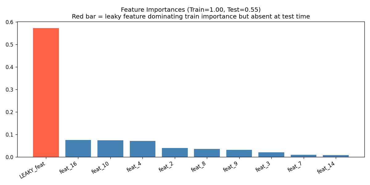
The red bar in Figure 8 is the diagnostic. One feature having an importance two to three times larger than the next — especially when combined with the train/test gap shown in the title — is the leakage signature. In a real project, that feature name goes straight onto the investigation list.
Common real-world leakage sources:
- Target-mean encoding computed before train/test split
- Timestamps or IDs that correlate with outcome ordering
- Features derived from post-outcome administrative events
- Join keys that inadvertently pull in outcome-adjacent tables
Diagnostic 9: The Full Diagnosis Report — A One-Call Sanity Check
The previous eight diagnostics each answer a specific question. For day-to-day use, you want a single function that gives you a structured verdict without requiring you to remember the full workflow. I built full_diagnosis() for exactly this purpose.
def full_diagnosis(model, X, y, model_name="Model"):
    X_train, X_test, y_train, y_test = train_test_split(X, y, test_size=0.2)

    model.fit(X_train, y_train)
    train_acc = accuracy_score(y_train, model.predict(X_train))
    test_acc  = accuracy_score(y_test,  model.predict(X_test))
    cv_scores = cross_val_score(model, X_train, y_train, cv=10)
    gap       = train_acc - test_acc

    # Verdict logic: underfitting check first, then gap severity
    if train_acc < 0.78 and test_acc < 0.78:
        verdict = "UNDERFITTING ..."
    elif gap > 0.18:
        verdict = "SEVERE OVERFITTING ..."
    elif gap > 0.12:
        verdict = "MODERATE OVERFITTING ..."
    elif gap > 0.06:
        verdict = "MILD OVERFITTING ..."
    else:
verdict = "GOOD FIT ..."Running this on five classifiers:
╔══════════════════════════════════════════════════════════════╗
  OVERFITTING DIAGNOSIS — Deep Decision Tree (overfit)
  Train accuracy      : 1.0000
  Test accuracy       : 0.7750
  Train–Test gap      : 0.2250  ⚠ HIGH
  CV mean (10-fold)   : 0.7417
  CV std  (10-fold)   : 0.0705  ⚠ UNSTABLE
  Verdict: SEVERE OVERFITTING — reduce complexity, add regularization, get more data
╚══════════════════════════════════════════════════════════════╝

╔══════════════════════════════════════════════════════════════╗
  OVERFITTING DIAGNOSIS — Random Forest
  Train accuracy      : 1.0000
  Test accuracy       : 0.9333
  Train–Test gap      : 0.0667  ✓ OK
  CV mean (10-fold)   : 0.8958
  CV std  (10-fold)   : 0.0280  ✓ STABLE
  Verdict: MILD OVERFITTING — monitor, may be acceptable in some cases
╚══════════════════════════════════════════════════════════════╝

╔══════════════════════════════════════════════════════════════╗
  OVERFITTING DIAGNOSIS — Decision Stump (underfit)
  Train accuracy      : 0.7708
  Test accuracy       : 0.7000
  Train–Test gap      : 0.0708  ✓ OK
  CV mean (10-fold)   : 0.7604
  CV std  (10-fold)   : 0.0553  ✓ STABLE
  Verdict: UNDERFITTING — increase model complexity, add better features
╚══════════════════════════════════════════════════════════════╝
Two things worth noting in the verdict logic. First, the underfitting check runs before the gap check — a decision stump has a small gap and stable CV, but both scores are low. Without the absolute-accuracy gate, it would pass as a “good fit.” Second, the Random Forest shows train=1.0 with a small test gap — this is typical behaviour for bagged ensembles and is usually acceptable. The key number is the test accuracy, not the train accuracy.
Key Takeaways
Pulling everything together, here is the diagnostic workflow I’ve settled on:
Start with learning curves. They answer the most fundamental question — is the problem high bias or high variance — and that answer determines every subsequent decision. If the gap is large, more data or regularisation. If both scores are low, more model capacity or better features.
Use validation curves to tune hyperparameters. Don’t grid-search blindly. Plot the validation curve first; it tells you the direction of the optimum and the sensitivity of performance to the parameter. You’ll waste far fewer compute cycles.
Monitor CV standard deviation, not just the mean. A model with high CV std is an unstable model. It may get lucky on your test split. It will not get lucky in production.
Treat near-perfect train accuracy with suspicion. It is almost never a sign that you’ve built a perfect model. It is usually a sign of overfitting, leakage, or both. The feature importance plot is the fastest way to distinguish them.
Apply the bias–variance decomposition to understand which lever to pull. Bias-dominated error → increase capacity, add features. Variance-dominated error → regularise, get more data, use an ensemble.
Regularise aggressively on high-dimensional regression. Ridge and Lasso are fast, interpretable, and almost always improve the generalisation gap when n_features > n_samples / 10.
Wire full_diagnosis() into your training script. Make the diagnostic automated so you can’t forget to run it. A two-second sanity check at the end of every training run will catch the majority of problems before they reach a reviewer.
What’s Coming in Part 2
Part 2 of this series will cover class imbalance — a different but related failure mode where models that look healthy on standard metrics are quietly useless on the minority class. We’ll examine precision-recall curves, calibration plots, and threshold selection strategies. The diagnostic mindset is the same; the tools differ.
Code Availability
The complete code for all nine diagnostics (app.py) is self-contained and requires only standard scientific Python libraries. All random states are fixed at seed=42 for reproducibility. The nine output figures are saved as numbered PNGs in the working directory.
Complete code: https://github.com/Emmimal/ml-diagnostics-overfitting/
Disclosure
All experiments in this article were designed and run by the author. The code was written from scratch for this article and does not incorporate proprietary data or models. Synthetic datasets were generated using scikit-learn’s built-in generators with no real-world data involved.
The author has no financial relationship with any of the libraries referenced. All tools mentioned are open-source.
The code, output, and analysis are the author’s own work.
Further Exploration
If this article got you thinking more carefully about model behaviour, these are worth reading next:
Feature Engineering in Machine Learning — Overfitting and underfitting are often symptoms of what happened before training. This piece covers how to build features that give your model something real to learn from, which is the upstream fix for half the bias problems in Diagnostic 6.
Top 6 Regression Techniques — Once you can diagnose the generalisation gap, the next question is which model family to reach for. A good companion to the Ridge and Lasso section in Diagnostic 7.
Handle Missing Values in Data Science — Missing value imputation is one of the most common sources of the data leakage pattern shown in Diagnostic 8. Worth reading alongside that section.
Machine Learning Algorithms — A broader map of the algorithm landscape. Useful context for understanding why different model families sit in different parts of the bias-variance spectrum covered in Diagnostic 6.
References
[1] Pedregosa, F., et al. (2011). Scikit-learn: Machine Learning in Python. Journal of Machine Learning Research, 12, 2825–2830. https://jmlr.org/papers/v12/pedregosa11a.html
[2] scikit-learn developers. (2024). scikit-learn 1.4 documentation. https://scikit-learn.org/stable/
[3] Harris, C.R., et al. (2020). Array programming with NumPy. Nature, 585, 357–362. https://doi.org/10.1038/s41586-020-2649-2
[4] Hunter, J.D. (2007). Matplotlib: A 2D graphics environment. Computing in Science & Engineering, 9(3), 90–95. https://doi.org/10.1109/MCSE.2007.55
[5] Prechelt, L. (1998). Early Stopping — But When? In Neural Networks: Tricks of the Trade, Lecture Notes in Computer Science, vol. 1524. Springer, Berlin, Heidelberg. https://doi.org/10.1007/3-540-49430-8_3
[6] Chollet, F., et al. (2015). Keras. https://keras.io
[7] Falcon, W., et al. (2019). PyTorch Lightning. https://www.pytorchlightning.ai
[8] Breiman, L. (2001). Random Forests. Machine Learning, 45(1), 5–32. https://doi.org/10.1023/A:1010933404324
[9] Geman, S., Bienenstock, E., & Doursat, R. (1992). Neural Networks and the Bias/Variance Dilemma. Neural Computation, 4(1), 1–58. https://doi.org/10.1162/neco.1992.4.1.1
[10] Efron, B., & Tibshirani, R. (1994). An Introduction to the Bootstrap. Chapman & Hall/CRC.
[11] Raschka, S. (2018). MLxtend: Providing machine learning and data science utilities and extensions to Python’s scientific computing stack. The Journal of Open Source Software, 3(24). https://doi.org/10.21105/joss.00638
[12] Kohavi, R., & Wolpert, D.H. (1996). Bias Plus Variance Decomposition for Zero-One Loss Functions. In Proceedings of the 13th International Conference on Machine Learning (ICML). Morgan Kaufmann.
[13] Tibshirani, R. (1996). Regression Shrinkage and Selection via the Lasso. Journal of the Royal Statistical Society: Series B (Methodological), 58(1), 267–288. https://doi.org/10.1111/j.2517-6161.1996.tb02080.x
[14] Hastie, T., Tibshirani, R., & Friedman, J. (2009). The Elements of Statistical Learning: Data Mining, Inference, and Prediction (2nd ed.). Springer. https://doi.org/10.1007/978-0-387-84858-7
[15] Kaufman, S., Rosset, S., Perlich, C., & Stitelman, O. (2012). Leakage in Data Mining: Formulation, Detection, and Avoidance. ACM Transactions on Knowledge Discovery from Data, 6(4), 1–21. https://doi.org/10.1145/2382577.2382579
Part 1 of the ML Diagnostics Mastery series. Follow for Part 2: Class Imbalance — When Accuracy Lies.


 in Generative Music: A New Era of Creativity")

Leave a Reply