

PyTorch Debugging Checklist: A Systematic Framework to Fix Models That Won’t Learn
This is not another “try lowering your learning rate” guide. This is a systematic debugging framework used to diagnose exactly why neural networks fail to learn — with reproducible checks, real terminal output, and production-grade practices built in from the start.
If your model is stuck at 10% accuracy, your loss isn’t decreasing, or you’re staring at a flat curve convinced the GPU is broken — this guide will help you find the exact reason. Not guess at it.
The Problem With How Most People Debug Neural Networks
Most deep learning practitioners debug the same way: change something, rerun training, wait 20 minutes, see if it got better, repeat. No structure. No isolation. No baseline.
This is expensive and unreliable. A training run that takes 20 minutes to tell you “still broken” is 20 minutes you could have spent actually fixing the bug — if you knew what it was.
The bugs that kill neural network training sessions are almost never exotic. They’re not your architecture. They’re not your dataset size. They’re silent, boring mistakes: a normalization applied twice, a learning rate off by two orders of magnitude, a model.eval() that never switched back to model.train(). They hide because nothing crashes — the script runs, loss is computed, gradients flow — just uselessly.
If your model is stuck at random accuracy (10% for a 10-class problem), or your loss curve is flat, or your validation loss is inexplicably higher than expected — work through this checklist in order. Stop at the first failure. Fix it before moving on.
The framework is structured as a pyramid of trust: before you can trust your training, you have to trust your evaluation. Before you can trust your evaluation, you have to trust your optimization. Before you trust any of that, you have to trust your data.
Complete code: https://github.com/Emmimal/pytorch-debugging-checklist/
The Debug Pyramid: Build From the Ground Up
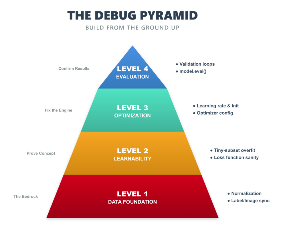
The pyramid has four levels:
Level 1 — Data (foundation): Are your inputs sane? Is normalization correct? Do labels match images? Nothing above this works if the foundation is broken.
Level 2 — Learnability: Can this model, with this loss function, learn anything at all? The tiny-subset overfit test answers this definitively.
Level 3 — Optimization: Is your learning rate in the right ballpark? Are your weights initialized without symmetry? Is your optimizer set up correctly for the task?
Level 4 — Evaluation (apex): Is your validation loop correct? Are you using model.eval()? Does per-class accuracy look uniform? Are there systematic confusion pairs?
Each level depends on the one below it. A broken optimization layer will produce bad evaluation numbers, but fixing the evaluation won’t help — you have to fix the optimization. That’s why the order matters.
The Setup: Environment and Model
All checks in this article use a simple two-layer CNN on MNIST. The simplicity is intentional: if this model can’t learn MNIST, something is fundamentally broken in your setup — not your architecture, not your dataset. Calibrate here, then scale up.
BATCH_SIZE  = 512
NUM_EPOCHS  = 10
DEVICE      = torch.device("cuda" if torch.cuda.is_available() else "cpu")
SEED        = 42
torch.manual_seed(SEED)class SimpleCNN(nn.Module):
"""
Input → Conv(1→32, 3×3) → ReLU → MaxPool(2)
→ Conv(32→64, 3×3) → ReLU → MaxPool(2)
→ Flatten → FC(3136→128) → ReLU → Dropout(0.3)
→ FC(128→10) [raw logits — CrossEntropyLoss handles softmax]
"""
def __init__(self):
super().__init__()
self.conv1 = nn.Conv2d(1, 32, kernel_size=3, padding=1)
self.conv2 = nn.Conv2d(32, 64, kernel_size=3, padding=1)
self.pool = nn.MaxPool2d(2)
self.fc1 = nn.Linear(64 * 7 * 7, 128)
self.fc2 = nn.Linear(128, 10)
self.dropout = nn.Dropout(0.3)
def forward(self, x):
x = self.pool(F.relu(self.conv1(x))) # 28→14
x = self.pool(F.relu(self.conv2(x))) # 14→7
x = x.view(x.size(0), -1) # flatten: 64×7×7 = 3136
x = F.relu(self.fc1(x))
x = self.dropout(x)
return self.fc2(x) # raw logits421,642 trainable parameters. More than enough for MNIST. If this fails to learn, the problem is in your setup — not the model.
Final result: 99.10% validation accuracy in 10 epochs, on CPU.
CHECK 1: Data Pipeline — “Are My Inputs Actually Sane?”
The most common source of silent bugs in deep learning is also the least glamorous: your data pipeline.
The failures look like: normalization applied twice, a random shuffle that decouples labels from images, a transform that zeroes every tensor, pixel values left in [0, 255] instead of [-1, 1]. None of these crash your script. All of them will make your model fail to learn, and you’ll spend days blaming the architecture.
Always inspect raw samples before a single gradient is computed.
transform = T.Compose([
    T.ToTensor(),
    T.Normalize((0.1307,), (0.3081,))   # MNIST channel mean & std
])

images, labels = next(iter(train_loader))

# Shape check
assert images.shape == (BATCH_SIZE, 1, 28, 28), f"Unexpected: {images.shape}"

# Value range — post-normalization must be centred near 0
mean_val = images.mean().item()
if not (-1.0 < mean_val < 1.0):
    raise RuntimeError(f"Image mean is {mean_val:.3f}. Did you normalize?")

# Label range
assert labels.min() >= 0 and labels.max() <= 9Actual output from the run:
✓  Image shape correct: (512, 1, 28, 28)
✓  Image stats: mean=-0.001, std=0.998
✓  Labels in [0, 9] — classes seen: [0, 1, 2, 3, 4, 5, 6, 7, 8, 9]
✓  All 10 classes present in first batch
A mean of -0.001 and std of 0.998 confirm normalization is working. Always pair the programmatic checks with a visual grid — it takes 30 seconds and catches label mismatches the assertions miss.
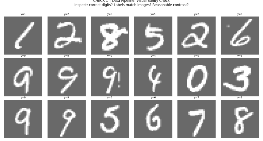
What to look for:
- Are the digit labels consistent with what you see?
- Do the images have reasonable contrast? (All black or all white = broken normalization.)
- Are any images clearly corrupted or blank?
CHECK 2: Broken Baseline — “What Does Failure Actually Look Like?”
Before you can recognize a broken model, you need to know what broken looks like. This is the step most tutorials skip. It’s the most important one.
We deliberately train a broken model: zero-initialized weights combined with an absurd learning rate of 10.0. The zero-init creates the gradient symmetry problem — every neuron in a layer receives the same gradient and updates identically. The model effectively has one neuron per layer regardless of width. The high learning rate ensures that even if gradients flow, the updates will be catastrophic.
class BrokenCNN(nn.Module):
    def __init__(self):
        super().__init__()
        # Same architecture — different init
        for m in self.modules():
            if isinstance(m, (nn.Conv2d, nn.Linear)):
                nn.init.constant_(m.weight, 0.0)   # symmetry problem
                nn.init.constant_(m.bias,   0.0)

broken_optim = torch.optim.SGD(broken_model.parameters(), lr=10.0) # absurdActual output:
✓ Broken model confirmed stuck at ~10.0% (≈ random chance for 10 classes)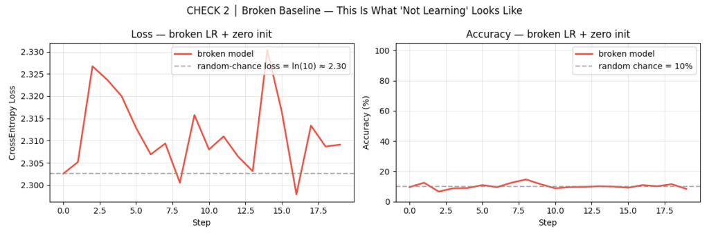
Commit the following failure signatures to memory. When you see them in a real training run, you now know exactly where to look:
| Symptom | Likely Cause |
|---|---|
| Loss stuck at ln(10) ≈ 2.30 | Zero or symmetric weight initialization |
| Loss exploding to NaN or Inf | Learning rate is catastrophically high |
| Loss drops briefly then plateaus | LR too low, or architecture bottleneck |
| ~10% accuracy throughout | Model is predicting one class for every input |
| Val loss much higher than train loss | model.eval() not called during validation |
CHECK 3: Overfit a Tiny Subset — “Can This Model Learn Anything at All?”
This is the single most powerful debugging technique in deep learning. Before running on your full dataset, pick 50 samples and drive the training loss to zero. If you can’t do this, your model, loss function, or data has a fundamental bug.
Why 50 samples? It’s small enough to overfit in seconds, but large enough to exercise your full pipeline — data loading, model forward pass, loss computation, backward pass, weight update. If any of these components is broken, this test will catch it.
tiny_loader = DataLoader(
    Subset(train_dataset, range(50)),
    batch_size=16,
    shuffle=True
)
tiny_optim  = torch.optim.Adam(model.parameters(), lr=1e-3)
TARGET_LOSS = 0.01   # success threshold

for epoch in range(50):
    for imgs, lbls in tiny_loader:
        imgs, lbls = imgs.to(DEVICE), lbls.to(DEVICE)
        tiny_optim.zero_grad()
        loss = criterion(model(imgs), lbls)
        loss.backward()
        tiny_optim.step()

    if avg_loss < TARGET_LOSS:
        print(f"Converged at epoch {epoch+1}")
        break
else:
    raise RuntimeError(
        "Could not overfit 50 samples. "
        "Fix this before training on the full dataset."
)Actual output:
  Epoch  10 | Loss: 0.482603
  Epoch  20 | Loss: 0.071965
  Epoch  30 | Loss: 0.016749
  ✓  Converged at epoch 34 — loss=0.008187 < 0.01
  ✓  Final tiny-subset accuracy: 100.0%  (expect 100%)
  ✓  Architecture is capable of learning — proceed to full training.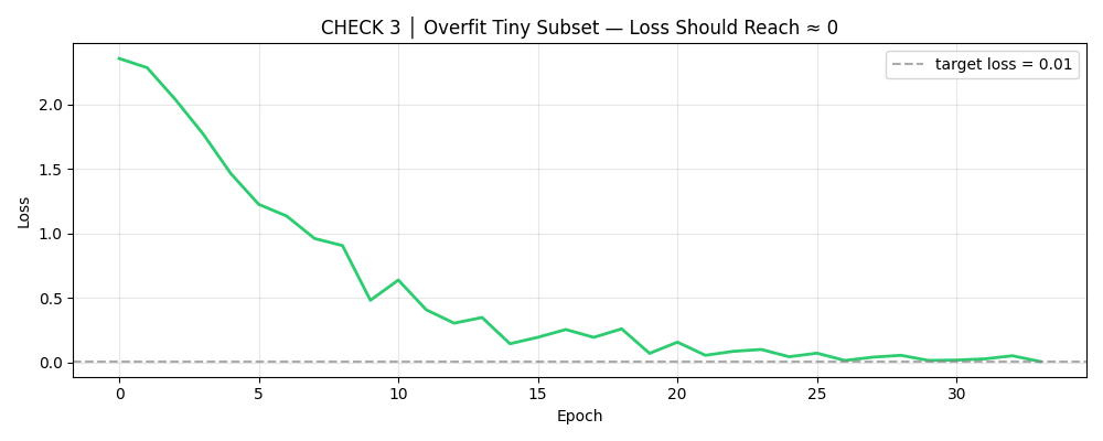
If this check fails, possible causes include:
- A dead ReLU that kills gradient flow in the first layer
- A loss function that doesn’t depend on your model’s parameters (a disconnected computation graph — happens with detached tensors)
- Labels that don’t match images in the tiny subset
- A skip connection or residual path that bypasses the learnable weights entirely
Do not skip this check even if you’re in a hurry. A model that fails here has no business running on your full dataset.
CHECK 4: Learning Rate Finder — “Am I Even in the Right Ballpark?”
The learning rate is the single most important hyperparameter in neural network training, and the one most often chosen by guessing. A learning rate that’s too high will cause your loss to explode or bounce chaotically. A learning rate that’s too low will cause your loss to stagnate for dozens of epochs before making any progress. The right learning rate varies by architecture, batch size, optimizer, and data — there’s no universal default.
The LR range test, introduced by Leslie Smith in 2015 and popularized by fast.ai, gives you a principled estimate in one epoch.
The algorithm: Sweep the learning rate from a very small value (1e-6) to a large one (10.0) over 100-200 steps. At each step, record the smoothed loss. Plot loss vs. learning rate on a log scale. The suggested learning rate sits just before the loss begins to rise sharply — in the steepest, most stable descent.
Several important refinements over the naive implementation:
High EMA smoothing (β = 0.9): The raw loss is too noisy to read directly. Exponential moving average with β = 0.9 smooths it into a clean curve without lagging too far behind.
Skip the warmup (first 15%): The earliest steps have unstable loss because the EMA hasn’t converged yet. Searching in this region always suggests a near-zero LR.
The “valley” rule instead of steepest descent: Find the loss minimum in the search window, then step back one decade (÷ 10) on the log scale. This is more robust than finding the steepest gradient under heavy smoothing — with high β, the curve can be nearly flat for the first half, making noise dominate the derivative.
suggested_lr = find_lr(
    model, train_loader, criterion,
    start_lr  = 1e-6,
    end_lr    = 10.0,     # wide sweep to see the full descent+explosion arc
    num_iter  = 200,      # fine resolution on the log scale
    smooth    = 0.9,
    skip_frac = 0.15,
    clip_frac = 0.75,
    lr_min    = 1e-4,     # safety floor
    lr_max    = 1e-1,     # safety ceiling
)Actual output:
✓ Suggested LR: 1.11e-04 (loss minimum ÷ 10 — one safe decade back)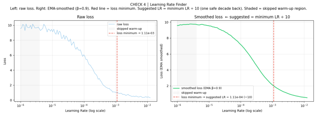
When the LR finder misbehaves: If the smoothed curve has no clear minimum (it only goes down, or only goes up), widen your sweep (end_lr = 100.0) or increase num_iter to 300 for finer resolution. If the suggested LR gets clamped by the safety bounds, check whether your batch size is large enough to produce a stable gradient signal.
CHECK 5: Weight Initialization — “Did My Weights Start in a Good Place?”
Default PyTorch initialization is reasonable but not optimal. Explicitly applying Kaiming (He) initialization for ReLU networks gives more stable early gradients, and — critically — breaks the symmetry that zero-init causes.
The math: Kaiming normal initialization sets each layer’s weight variance to 2/fan_in, which preserves the expected variance of activations through ReLU layers. Without this, activations either vanish (shrinking toward zero through depth) or explode (growing uncontrollably). Either state makes early gradients near-zero and training extremely slow.
For Sigmoid or Tanh activations, use Xavier initialization (nn.init.xavier_normal_) instead — it accounts for the different saturation characteristics of those functions.
def init_weights(m: nn.Module):
    if isinstance(m, (nn.Conv2d, nn.Linear)):
        nn.init.kaiming_normal_(m.weight, mode="fan_out", nonlinearity="relu")
        if m.bias is not None:
            nn.init.constant_(m.bias, 0.0)

model.apply(init_weights)Actual output:
✓  conv1.weight — mean=-0.0038, std=0.0867  (expect ~0 mean)
✓  Weight std in healthy range.
✓  Kaiming initialization applied and verified.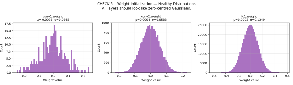
The diagnostic thresholds:
std < 0.01: Vanishing gradient risk — weights start too small, gradients will be near zero in the first few stepsstd > 1.0: Exploding gradient risk — early updates will be catastrophically largemean ≠ ~0: Asymmetric initialization — neurons in the same layer will start with different biases, which can cause class-specific failure modes
CHECK 6: Full Training Loop — “Does Everything Actually Come Together?”
Now we assemble the production-grade training loop. Three decisions are worth explaining in detail.
AdamW, not Adam
The standard Adam optimizer has a subtle but important bug: weight decay is applied to the gradient update rather than directly to the weights, which interacts incorrectly with the adaptive learning rate scaling. AdamW (Loshchilov & Hutter, 2019) fixes this decoupling. On simple problems like MNIST the difference is small; on transformer models and larger architectures it matters considerably.
OneCycleLR scheduler
A flat learning rate wastes the early and late phases of training. OneCycleLR applies a warmup phase (the first 30% of training), ramps to a maximum LR, then anneals with cosine decay. The warmup prevents catastrophically large weight updates in epoch 1, when gradients are noisiest. The cosine annealing allows fine-grained convergence at the end.
Gradient clipping
torch.nn.utils.clip_grad_norm_(parameters, max_norm=1.0) prevents a single bad batch from producing a catastrophic weight update. It’s cheap, always safe, and protects against occasional gradient spikes in both early training and near batch boundaries.
optimizer = torch.optim.AdamW(
    model.parameters(),
    lr=suggested_lr,          # from LR finder: 1.11e-04
    weight_decay=1e-4,        # AdamW decouples this from gradient step
)

scheduler = OneCycleLR(
    optimizer,
    max_lr=suggested_lr * 10,  # 10× headroom — OneCycleLR needs room to ramp
    steps_per_epoch=len(train_loader),
    epochs=NUM_EPOCHS,
    pct_start=0.3,             # 30% spent warming up
    anneal_strategy="cos",     # cosine annealing
    div_factor=25.0,           # initial LR = max_lr / 25
    final_div_factor=1000.0,   # final LR = max_lr / 1000
)A critical detail many engineers miss: model.eval() does two things. It disables dropout. And it switches BatchNorm layers from batch statistics to running statistics. Forgetting this during validation inflates your validation loss and makes your model appear to overfit when it isn’t. Always call model.eval() before the validation loop, and model.train() before the training loop.
Actual training output:
  Epoch   Train Loss   Val Loss    Val Acc     Time
  ──────────────────────────────────────────────────────────────
      1       4.3095     0.3303     90.24%   74.8s
      2       0.2894     0.1078     96.83%   77.0s
      3       0.1327     0.0585     97.99%   78.5s
      4       0.0822     0.0427     98.64%   79.7s
      5       0.0616     0.0377     98.80%   79.6s
      6       0.0484     0.0318     98.97%   78.6s
      7       0.0362     0.0302     99.03%   82.6s
      8       0.0301     0.0282     99.11%   79.5s
      9       0.0261     0.0278     99.07%   81.0s
     10       0.0242     0.0277     99.10%   80.0s
Notice epoch 1’s high train loss (4.31) despite a decent val loss (0.33). This is OneCycleLR’s warmup working correctly — the model starts with a very small LR (max_lr / 25 = 4.4e-5), so training epoch 1 updates are tiny. But the Kaiming-initialized weights already place the model in a reasonable starting configuration, which is why val loss is meaningful even before real optimization begins.
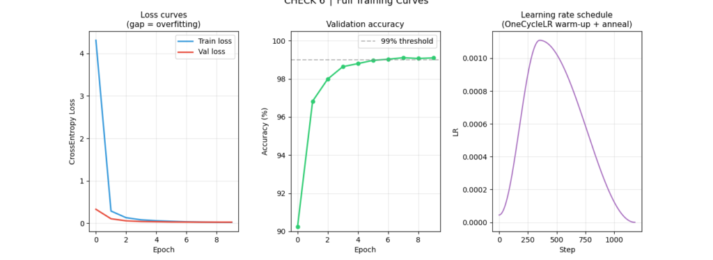
Reading the training table:
- Train loss dropping rapidly each epoch: the model is learning, gradients are healthy
- Val loss converging alongside train loss: no significant overfitting
- Val accuracy approaching 99%: close to the practical performance ceiling for this architecture
- The slight increase in val loss at epoch 9 (0.0278) vs epoch 8 (0.0282) is within noise — the early stopping note in the code flags it but doesn’t trigger
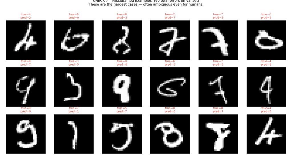
CHECK 7: Final Debug Dashboard — “Did the Model Learn Uniformly?”
A model that achieves 99% overall accuracy but predicts only 9 of the 10 classes correctly could still hit 90% — depending on class distribution. Per-class breakdown and the confusion matrix reveal what the aggregate metric hides.
Actual final results:
  Final Val Accuracy  : 99.10%
  Best Val Accuracy   : 99.11%  (epoch 8)
  Final Train Loss    : 0.0242
  Final Val Loss      : 0.0277
  Generalisation Gap  : 0.0034  (healthy)

  Per-class accuracy:
    digit 0:  99.39%  ████████████████████████████████████████████████
    digit 1:  99.82%  ████████████████████████████████████████████████
    digit 2:  99.22%  ████████████████████████████████████████████████
    digit 3:  99.70%  ████████████████████████████████████████████████
    digit 4:  99.08%  ████████████████████████████████████████████████
    digit 5:  98.88%  ████████████████████████████████████████████████
    digit 6:  98.54%  ████████████████████████████████████████████████
    digit 7:  99.03%  ████████████████████████████████████████████████
    digit 8:  98.67%  ████████████████████████████████████████████████
    digit 9:  98.51%  ████████████████████████████████████████████████
A generalization gap of 0.0034 is extremely healthy. No digit is below 98.5% — no class collapse, no systematic imbalance.
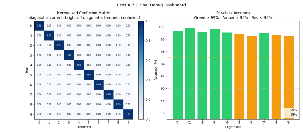
What to look for:
- Any off-diagonal cell in the confusion matrix that’s notably bright: systematic class confusion, possibly from poor feature separation or imbalanced training data for that class
- Any bar in the per-class chart that’s amber or red: consider augmenting samples of that class, applying class-weighted loss, or investigating whether the class’s training samples are lower quality
- Patterns in the misclassified examples: are they ambiguous to humans too? If yes, the model is at its ceiling. If no, the model has a fixable failure mode.
The 5 Bugs This Checklist Was Designed to Catch
These are the most common silent killers of neural network training sessions:
1. Forgetting model.eval() and model.train() Dropout and BatchNorm behave differently in training vs. inference mode. Running dropout during evaluation inflates validation loss. Running BatchNorm in training mode during evaluation leaks batch statistics. Both make your model appear to overfit when it isn’t. Check 7 catches this by comparing train and val loss curves; Check 6’s code comments flag exactly where these calls are required.
2. Learning rate off by an order of magnitude lr=0.01 vs lr=0.001 is the difference between divergence and convergence. The LR finder in Check 4 gives you a principled estimate instead of a guess. Run it once for each new architecture and dataset combination.
3. Zero or symmetric weight initialization All neurons in a layer receive the same gradient signal and update identically. The network has effectively one neuron per layer regardless of stated width. Check 2 shows you what this looks like in training curves; Check 5 applies the fix.
4. Unnormalized or improperly scaled inputs Pixel values in [0, 255] instead of [-1, 1] produce a poorly conditioned loss landscape. Convergence is slow or impossible. Check 1 verifies mean and standard deviation before any gradient is computed.
5. Data/label mismatch A random.shuffle on images but not labels. An off-by-one in dataset indexing. A DataLoader that processes images and labels with different random seeds. None of these crash your script — they just make your labels wrong. Check 1’s visual grid catches this in under 60 seconds.
Debugging Toolkit: Copy-Paste Ready
The five most useful snippets from the full script, ready to drop into any PyTorch project:
Snippet 1: Data sanity check
def check_data_pipeline(loader, n_classes=10):
    images, labels = next(iter(loader))
    mean_val = images.mean().item()
    std_val  = images.std().item()

    print(f"Shape : {tuple(images.shape)}")
    print(f"Mean  : {mean_val:.3f}  (expect near 0 after normalization)")
    print(f"Std   : {std_val:.3f}  (expect near 1 after normalization)")
    print(f"Labels: {sorted(labels.unique().tolist())}")

    if not (-1.0 < mean_val < 1.0):
        raise RuntimeError(f"Image mean {mean_val:.3f} out of range — check normalization.")
    if labels.min() < 0 or labels.max() >= n_classes:
        raise RuntimeError(f"Labels out of range: [{labels.min()}, {labels.max()}]")
print("✓ Data pipeline check passed.")Snippet 2: Tiny-subset overfit test
def can_overfit(model, dataset, criterion, device, n_samples=50,
                max_epochs=50, target_loss=0.01, lr=1e-3):
    loader = DataLoader(Subset(dataset, range(n_samples)), batch_size=16, shuffle=True)
    optim  = torch.optim.Adam(model.parameters(), lr=lr)

    model.train()
    for epoch in range(max_epochs):
        total_loss = 0.0
        for imgs, lbls in loader:
            imgs, lbls = imgs.to(device), lbls.to(device)
            optim.zero_grad()
            loss = criterion(model(imgs), lbls)
            loss.backward()
            optim.step()
            total_loss += loss.item()
        avg = total_loss / len(loader)
        if avg < target_loss:
            print(f"✓ Overfit in {epoch+1} epochs (loss={avg:.5f})")
            return True
raise RuntimeError(f"Could not overfit {n_samples} samples (loss={avg:.4f}). Fix architecture/loss first.")Snippet 3: LR finder (standalone, drop-in)
def find_lr(model, loader, criterion, device,
            start_lr=1e-6, end_lr=10.0, num_iter=100,
            smooth=0.9, skip_frac=0.10, clip_frac=0.80):
    import math
    from torch.optim.lr_scheduler import LambdaLR

    optimizer = torch.optim.Adam(model.parameters(), lr=start_lr)
    scheduler = LambdaLR(optimizer,
        lambda x: math.exp(x * math.log(end_lr / start_lr) / num_iter))

    lrs, smoothed, avg_loss, best = [], [], None, float("inf")

    model.train()
    for i, (imgs, lbls) in enumerate(loader):
        if i >= num_iter: break
        imgs, lbls = imgs.to(device), lbls.to(device)
        optimizer.zero_grad()
        loss = criterion(model(imgs), lbls)
        loss.backward()
        optimizer.step()

        raw      = loss.item()
        avg_loss = raw if avg_loss is None else smooth * avg_loss + (1 - smooth) * raw
        lrs.append(optimizer.param_groups[0]["lr"])
        smoothed.append(avg_loss)
        scheduler.step()

        if avg_loss < best: best = avg_loss
        if avg_loss > 4 * best and i > 10: break

    n     = len(smoothed)
    skip  = max(1, int(n * skip_frac))
    clip  = max(skip + 2, int(n * clip_frac))
    region = smoothed[skip:clip]
    min_idx = region.index(min(region)) + skip
return lrs[min_idx] / 10.0 # one decade before minimumSnippet 4: Kaiming initialization (drop-in)
def init_kaiming(model: nn.Module):
    """
    Apply Kaiming He initialization to all Conv and Linear layers.
    Use for ReLU networks. Switch to xavier_normal_ for Tanh/Sigmoid.
    """
    for m in model.modules():
        if isinstance(m, (nn.Conv2d, nn.Linear)):
            nn.init.kaiming_normal_(m.weight, mode="fan_out", nonlinearity="relu")
            if m.bias is not None:
                nn.init.constant_(m.bias, 0.0)
    return model

model = init_kaiming(SimpleCNN().to(DEVICE))Snippet 5: Per-class accuracy from a validation loop
def per_class_accuracy(model, loader, device, n_classes=10):
    model.eval()
    conf = torch.zeros(n_classes, n_classes, dtype=torch.long)

    with torch.no_grad():
        for imgs, lbls in loader:
            preds = model(imgs.to(device)).argmax(1).cpu()
            for t, p in zip(lbls, preds):
                conf[t, p] += 1

    per_class = conf.diag().float() / conf.sum(1).float() * 100
    for cls, acc in enumerate(per_class):
        flag = "✓" if acc >= 95 else "⚠"
        print(f"  {flag} Class {cls}: {acc:.2f}%")

    worst = per_class.argmin().item()
    print(f"\n  Worst class: {worst} ({per_class[worst]:.2f}%)")
return per_classExtending This Framework to Your Own Problem
This checklist was demonstrated on MNIST, but the structure is domain-agnostic. Here’s how to adapt each check:
Different task (object detection, segmentation, regression, NLP): Check 1 still runs the same sanity assertions but adapts to your data format — bounding boxes, masks, sequences. Check 3 uses your actual task-specific loss — Dice loss, Focal loss, CTC loss. Check 7 uses the appropriate evaluation metric — mAP, IoU, MAE, WER.
Different modality (text, audio, tabular data, time series): Check 1 is the most important to adapt. For time series: verify that your validation split is temporal — no data leakage from future samples into training. For text: check vocabulary size, token id ranges, padding. For audio: check sample rate, normalization, spectrogram statistics.
Larger models (transformers, ResNets, diffusion models): Check 3 still applies — any model that can’t memorize 50 samples has a fundamental bug. Check 4 should use a longer sweep (num_iter=300+) and finer LR resolution. Check 5 may need to account for LayerNorm layers in addition to Conv and Linear. Check 6 benefits from gradient accumulation if batch size is memory-constrained.
Quick Reference: What Each Check Catches
Debug Pyramid Level 1 — DATA
  Check 1 │ Data Pipeline     → corrupted/unnormalized inputs, label mismatches

Debug Pyramid Level 2 — LEARNABILITY
  Check 2 │ Broken Baseline   → establishes what failure looks like (your reference)
  Check 3 │ Tiny Subset       → architecture bugs, dead gradients, wrong loss function

Debug Pyramid Level 3 — OPTIMIZATION
  Check 4 │ LR Finder         → LR too high or too low
  Check 5 │ Initialization    → zero-init symmetry problem, vanishing/exploding init

Debug Pyramid Level 4 — EVALUATION
  Check 6 │ Full Training     → underfitting, overfitting, unstable dynamics
  Check 7 │ Dashboard         → class collapse, systematic confusion pairs, error analysis
Run these in order. Stop at the first failure. Fix it before moving on.
A network that can’t overfit 50 samples has no business training on 50,000.
Conclusion: Debugging Is a Discipline, Not Intuition
Neural network bugs are not mysterious. They are predictable. The failures that eat days of debugging time — unnormalized inputs, wrong learning rates, symmetry-breaking initialization — have known signatures, known causes, and known fixes.
The seven-step checklist in this article doesn’t guarantee you’ll catch every bug on the first pass. But it guarantees you’ll stop guessing and start diagnosing. And that shift — from intuition to process — is the difference between an engineer who spends three days staring at a flat loss curve and one who finds the bug in twenty minutes.
Apply the checklist to MNIST first. Get the 99.1% baseline. Memorize what each check’s output looks like when everything is healthy. Then apply the same structure to your real problem. The checks adapt; the discipline doesn’t change.
At Emitech Logic, we focus on building production-grade ML systems — not just models that run, but models that behave predictably, fail informatively, and can be debugged when they don’t.
References
- Smith, L. N. (2015). Cyclical Learning Rates for Training Neural Networks. arXiv:1506.01186. — The original LR range test. https://arxiv.org/abs/1506.01186
- He, K., Zhang, X., Ren, S., & Sun, J. (2015). Delving Deep into Rectifiers: Surpassing Human-Level Performance on ImageNet Classification. — The Kaiming initialization paper. https://arxiv.org/abs/1502.01852
- Loshchilov, I. & Hutter, F. (2019). Decoupled Weight Decay Regularization. arXiv:1711.05101. — The AdamW paper. https://arxiv.org/abs/1711.05101
- Howard, J. & Gugger, S. Fastbook, Chapter 5: Image Classification. — The fast.ai “valley” LR rule and practical training methodology.
- Karpatti, A. (2019). A Recipe for Training Neural Networks. karpathy.github.io. — The blog post that popularized the tiny-subset overfit technique. https://gist.github.com/chicobentojr/d20dd040ff957d24d43a94cdf92e913e
Full source code available in the companion GitHub repository. Tested on Python 3.11, PyTorch 2.3, torchvision 0.18. Runs in ~15 minutes on CPU, ~3 minutes on GPU.
Complete code: https://github.com/Emmimal/pytorch-debugging-checklist/
Related Reads
After finishing this debugging checklist, you might also enjoy these hand-picked articles that build on similar foundations:
- How to Build a Neural Network from Scratch Using Python
Learn the fundamentals of implementing a neural network step-by-step in pure Python — the perfect starting point before you start debugging why it fails to train. - Rise of Neural Networks: Historical Evolution, Practical Understanding and Future Impact on Modern AI Systems
Get a deeper context on how neural networks evolved and why systematic training practices matter in real-world AI development. - Feature Engineering in Machine Learning
Strong data pipelines and proper feature preparation are the foundation of successful model training. This guide complements the first check in the debugging pyramid. - Machine Learning Algorithms
A clear overview of core ML algorithms that helps you understand where optimization and evaluation issues commonly arise.


")
: A Step-by-Step Guide")
Leave a Reply