

How to Build an ML Retraining Pipeline That Won’t Break in Production
An ML retraining pipeline is the backbone of any production machine learning system. Without a proper ML retraining pipeline, models degrade silently as data changes, leading to inaccurate predictions and real-world failures.
Series: Production ML Engineering — Article 03 of 15 (Cluster 1: Foundation & Pipeline)
Before you read this: This article is part of a 15-part series on building production-grade ML systems. If you haven’t read the series hub yet, start with the Production ML Engineering guide — it maps out the five pillars every production system rests on and explains where this article fits. Article 02 covered containerization and deployment; this article picks up the moment your model is live and asks: what happens when it needs to change?
Core Components of an ML Retraining Pipeline
About four months after deploying a fraud detection model, I opened the notes from our original deployment to kick off the first retraining cycle. The monitoring dashboard had been showing score drift for two weeks. PSI on two features had crossed the action threshold. Recall was down 18% from the Month 0 baseline.
The retraining “procedure” turned out to be a markdown file with six manual steps. Two of them referenced a Python environment that no longer existed. One said: ask Priya about the S3 path.
Priya had left the team in February.
This is not a story about bad documentation. It is a story about a category error that most ML teams make: they build a model deployment and call it a production ML system. The deployment gets the engineering attention. The retraining gets a comment in the README. And then six months later, when the model actually needs to change — and it will — the team discovers that “we have retraining capability” and “we have a retraining pipeline” are two completely different claims.
This article builds the second thing. A retraining pipeline that is automated, testable, drift-aware, and safe to run by anyone on the team — including the engineer who joined last week and has never touched the model before.
Complete Code: https://github.com/Emmimal/ml-retraining-pipeline/
What a Retraining Pipeline Actually Is
A retraining pipeline is not a script that calls model.fit() on new data. That is retraining. A retraining pipeline is the system that decides when to retrain, what data to use, validates that the new model is actually better, and deploys it safely — with a rollback path if it is not.
The distinction matters because each of those four responsibilities has failure modes that the others cannot compensate for. If you retrain on the wrong data window, you get a model that performs well on evaluation and poorly in production. If you skip validation, you deploy a model that is worse than the one it replaced, and you only find out from a cost report two weeks later. If you have no rollback path, a bad deployment is an incident rather than a five-second reversion.
Before writing a single line of code, the pipeline design looks like this:
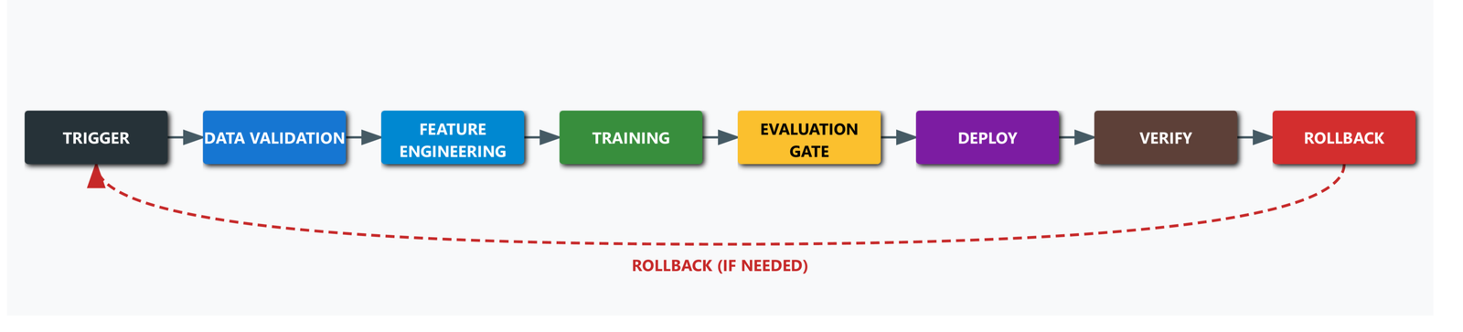
Every stage either passes its exit criteria and moves forward, or fails loudly and halts. There are no implicit steps. There is no tribal knowledge encoded in someone’s head or a markdown file.
When Should You Retrain?
The wrong answer is “when performance drops.” By the time performance has visibly degraded in production, you have already been absorbing the cost of that degradation for days or weeks. The right answer is: retrain before the degradation becomes operationally significant, using leading indicators.
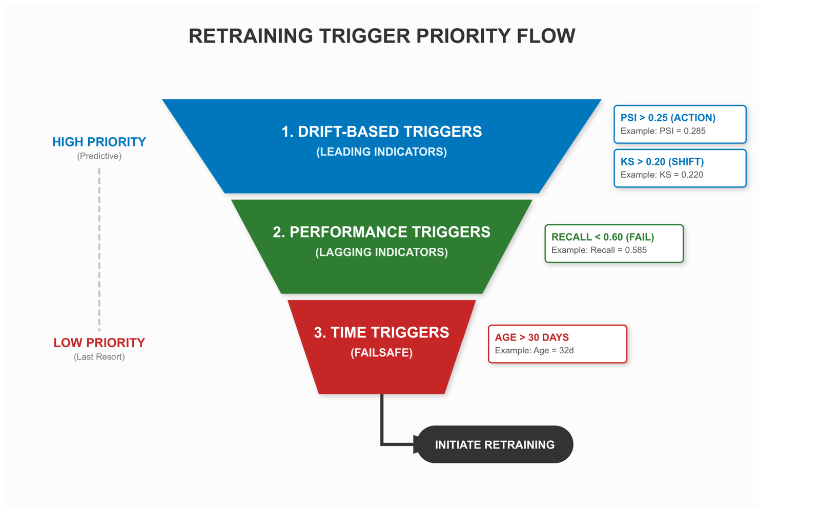
There are three trigger families, and each belongs at a different layer of the system.
Time-based triggers are simple and predictable — retrain every N days regardless of monitoring signals. The advantage is operational simplicity; every engineer on the team knows exactly when retraining happens. The disadvantage is that you retrain even when the data has not shifted, and you wait even when it has shifted dramatically. Time-based triggers are a failsafe, not a strategy.
Performance-based triggers fire when a metric crosses a threshold: recall drops below 0.65, cost per thousand transactions exceeds some business-defined limit. These are reactive — they respond to actual degradation — but they trigger after the damage has already begun. They are lagging indicators.
Drift-based triggers are the leading-indicator version. Fire retraining when PSI on key features crosses the action threshold, or when the KS statistic on the score distribution signals a distributional shift. These allow you to get ahead of performance degradation rather than respond to it (Gama et al., 2014).
In practice, a robust pipeline uses all three in combination, evaluated in priority order:
# pipeline/triggers.py

@dataclass
class TriggerConfig:
    max_days_since_training: int = 30    # time-based failsafe
    min_recall: float = 0.60             # performance-based (lagging)
    max_cost_per_1k: float = 15_000.0    # performance-based (lagging)
    psi_action_threshold: float = 0.25   # drift-based (leading)
    ks_action_threshold: float = 0.20    # drift-based (leading)

def should_retrain(..., config: TriggerConfig) -> tuple[bool, str]:
    # 1. Drift-based checks first — leading indicators
    flagged = {f: v for f, v in feature_psi.items()
               if v > config.psi_action_threshold}
    if flagged:
        worst = max(flagged, key=flagged.get)
        return True, f"PSI ACTION on '{worst}' (PSI={flagged[worst]:.3f})"

    ks_stat, _ = ks_2samp(ref_scores, cur_scores)
    if ks_stat > config.ks_action_threshold:
        return True, f"Score KS statistic elevated ({ks_stat:.3f})"

    # 2. Performance-based — lagging, but definitive
    if current_recall < config.min_recall:
        return True, f"Recall {current_recall:.3f} below minimum"

    # 3. Time-based — failsafe of last resort
    if days_since_training > config.max_days_since_training:
        return True, f"Model age ({days_since_training}d) exceeds maximum"

return False, "All checks passed — no retraining needed"The ordering is intentional. Drift fires first because it predicts degradation before it shows up in metrics. Performance fires second because it is lagging but definitive. Time fires last as a failsafe — even if nothing else triggers, the model gets refreshed on a known cadence.
The PSI thresholds here follow the standard classification from the statistical literature (Yurdakul, 2018): below 0.10 is stable, 0.10–0.25 warrants a warning, above 0.25 requires action.
Calibrating Your Thresholds
The values in TriggerConfig are not universal constants. The right approach is to look at historical monitoring data and find the PSI value at which recall had already dropped more than 10% from your baseline. That is your action threshold — the level at which retraining should have already started. Set your trigger just below it.
If you are starting from scratch with no historical monitoring data, the PSI literature thresholds are a reasonable starting point. Recalibrate after three months of production data.
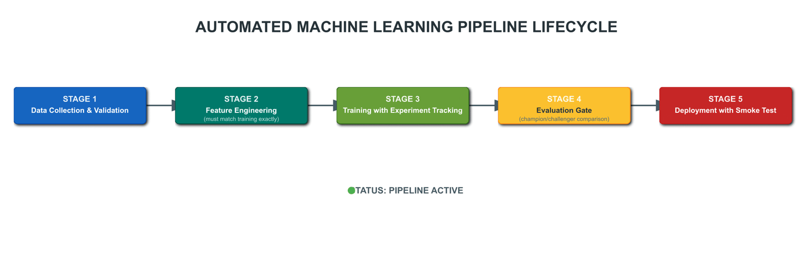
Let’s build each one.
Stage 1: Data Validation
The first thing that breaks in retraining pipelines is data. The lookback window is wrong, the schema has drifted, a feature that existed at original training time no longer exists upstream. Data validation is not optional — it is the gate that prevents all downstream stages from running on corrupt inputs (Breck et al., 2017).
The design choice that matters most here: accumulate all errors before raising, rather than stopping at the first failure. The engineer running a failed pipeline should see the complete picture in a single run, not fix one issue, re-run, discover the next issue, and repeat.
def validate_data(df: pd.DataFrame, config: DataConfig) -> None:
    errors = []

    if len(df) < config.min_samples:
        errors.append(f"Only {len(df)} samples — minimum is {config.min_samples}.")

    if "label" not in df.columns:
        errors.append("Column 'label' not found. Schema may have changed.")
    else:
        positive_rate = float(df["label"].mean())
        if positive_rate < config.min_positive_rate:
            errors.append(f"Positive rate {positive_rate:.4f} — suspiciously low.")
        if positive_rate > config.max_positive_rate:
            errors.append(f"Positive rate {positive_rate:.4f} — suspiciously high.")

    if config.required_features:
        missing = set(config.required_features) - set(df.columns)
        if missing:
            errors.append(f"Missing required features: {sorted(missing)}")

    # Null rate check — warn but do not block
    high_null = df.isnull().mean()[df.isnull().mean() > 0.10]
    if not high_null.empty:
        logger.warning("High null rates (>10%%) — will be imputed: %s", high_null.to_dict())

    if errors:
        raise DataValidationError(
            f"Data validation failed ({len(errors)} error(s)):\n" +
            "\n".join(f"  - {e}" for e in errors)
)Two design decisions worth explaining. First, the volume check rejects training on fewer than 500 samples by default. A model trained on an insufficient window will overfit to recent noise rather than learning durable patterns. The right minimum depends on your domain and class rarity — treat 500 as a floor, not a target. Second, the null rate check warns rather than fails. Upstream null issues often have legitimate causes — a feature added partway through the lookback window, a source that was temporarily unavailable. Silently failing every retrain run over a 12% null rate is worse than imputing and logging the warning.
Stage 2: Feature Engineering
This is where training-serving skew lives. The preprocessor that was fit at original training time — the StandardScaler, the SimpleImputer — must be applied with identical parameters at inference time. The way to enforce this is to load the same fitted artifact in both places, not to refit it from scratch on each retraining run (Sculley et al., 2015).
When retraining, you do refit the preprocessor — on the new data window. But the new preprocessor and the new model become artifacts that are versioned together, deployed together, and archived together. At no point does a model and a preprocessor from different training runs end up in the same serving environment.
def fit_and_save_preprocessor(df, artifact_dir):
    preprocessor = Pipeline([
        ("imputer", SimpleImputer(strategy="median")),
        ("scaler", StandardScaler()),
    ])
    X_transformed = preprocessor.fit_transform(df[FEATURE_COLS].values)
    joblib.dump(preprocessor, artifact_dir / "preprocessor.pkl")
return preprocessor, X_transformed, df["label"].valuesWhen the serving code loads preprocessor.pkl, it gets imputation and scaling in the correct order, fitted on the correct data window. There is no way to accidentally apply the wrong mean and variance — the artifact carries all of that state.
Stage 3: Training with Experiment Tracking
Every retraining run should produce a complete audit trail: which data window was used, what the git commit was, every hyperparameter, and the full evaluation suite for every candidate model. Three months from now, when something goes wrong in production, you need to reconstruct exactly what model was running and exactly what it was trained on.
The pipeline trains two candidate architectures — GradientBoostingClassifier and RandomForestClassifier — with 5-fold stratified cross-validation, and selects the winner by validation ROC-AUC. The full candidate comparison, not just the winner, is recorded in run_log.json.
{
  "run_id": "a3f1b2c4",
  "timestamp": "2025-04-14T02:17:43Z",
  "git_commit": "d4e8f1a",
  "data_window": "last_90_days",
  "winner_config": { "model_class": "GradientBoostingClassifier", ... },
  "cv_roc_auc_mean": 0.9312,
  "val_metrics": { "recall": 0.7241, "roc_auc": 0.9287, "cost_per_1k": 4823.0 },
  "all_candidates": [
    { "model_class": "GradientBoostingClassifier", "val_roc_auc": 0.9287 },
    { "model_class": "RandomForestClassifier",     "val_roc_auc": 0.9104 }
  ]
}This structure is intentionally compatible with MLflow and Weights & Biases logging APIs. If you are already using either, run_record feeds directly into their experiment tracking with minimal glue code.
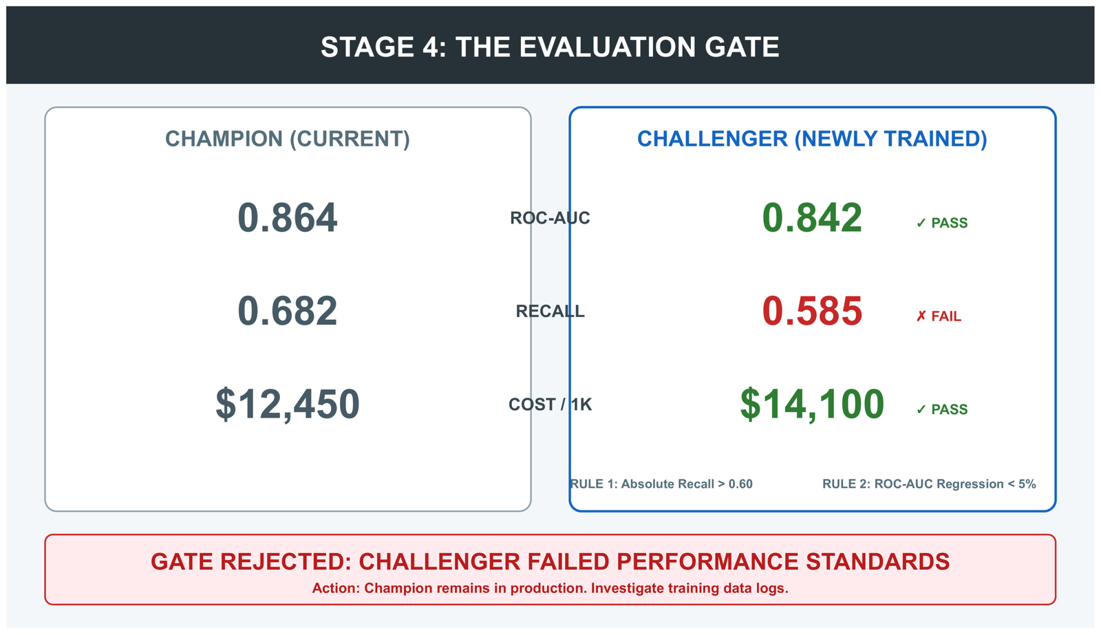
Stage 4: The Evaluation Gate
This is the stage most retraining scripts skip, and the one that causes the most production incidents in its absence.
The evaluation gate compares the challenger (the newly trained model) against the champion (the currently deployed model) on a held-out evaluation set. The challenger must clear two bars: it must meet absolute minimum performance standards, and it must not be significantly worse than the champion.
def run_evaluation_gate(challenger_model, X_eval, y_eval,
                        champion_artifact_dir, min_recall=0.60,
                        min_roc_auc=0.80, max_regression_pct=0.05):

    challenger_metrics = evaluate_model(challenger_model, X_eval, y_eval)
    champion_metrics = load_champion_metrics(champion_artifact_dir)
    failures = []

    # Rule 1: Absolute minimums — always required
    if challenger_metrics["recall"] < min_recall:
        failures.append(f"Recall {challenger_metrics['recall']:.4f} below minimum {min_recall}")
    if challenger_metrics["roc_auc"] < min_roc_auc:
        failures.append(f"ROC-AUC {challenger_metrics['roc_auc']:.4f} below minimum {min_roc_auc}")

    # Rule 2: No regression vs champion — required when a champion exists
    if champion_metrics is not None:
        regression = (champion_metrics["roc_auc"] - challenger_metrics["roc_auc"]) \
                     / champion_metrics["roc_auc"]
        if regression > max_regression_pct:
            failures.append(
                f"ROC-AUC regression {regression:.1%} exceeds allowed {max_regression_pct:.1%}"
            )

    if failures:
        raise EvaluationGateError("Challenger failed:\n" +
                                  "\n".join(f"  ✗ {f}" for f in failures))

return challenger_metricsThe 5% regression threshold is deliberately conservative. A challenger that is 5% worse than the champion should not be deployed — something went wrong in data collection, feature engineering, or training. It is better to keep the current model running while you investigate than to ship a regression automatically.
The first deployment gets a relaxed gate: absolute minimums only, with no champion to compare against. Every retrain after that is evaluated against the model it would replace. This asymmetry is intentional — it is easier to get into production than to stay in it, which is the correct incentive structure.
Stage 5: Deployment with Automatic Rollback
The deployment stage is intentionally thin. Full deployment machinery — containers, CI/CD, health checks — belongs in your deployment infrastructure. What this stage owns is the artifact promotion logic and the rollback path.
The promotion is a copy-swap, not a move:
def promote_artifacts(challenger_dir, production_dir):
    rollback_dir = production_dir.parent / "previous"

    # Archive current production before overwriting
    if production_dir.exists():
        if rollback_dir.exists():
            shutil.rmtree(rollback_dir)
        shutil.copytree(production_dir, rollback_dir)

    # Promote challenger
    if production_dir.exists():
        shutil.rmtree(production_dir)
    shutil.copytree(challenger_dir, production_dir)
    return rollback_dir


def rollback(rollback_dir, production_dir):
    if not rollback_dir.exists():
        raise RuntimeError("No rollback artifacts found.")
    if production_dir.exists():
        shutil.rmtree(production_dir)
shutil.copytree(rollback_dir, production_dir)The old artifacts stay in previous/ until the next promotion. At any point you can call rollback() and be back to the previous model in seconds. No network call. No registry lookup. No manual intervention. The rollback is a local file copy.
After promotion, the pipeline polls /health until the service confirms model_loaded: true. If the smoke test fails within the retry budget, rollback fires automatically. A bad deployment becomes a five-second reversion, not an incident.
Testing Your Pipeline Before You Need It
A retraining pipeline that has never been tested under failure conditions is not reliable — it is untested. The test suite covers three categories:
Stage failures: Each stage must fail loudly and halt correctly when given bad inputs. The data validation tests confirm that insufficient samples, missing labels, low positive rates, and missing features all raise DataValidationError with a message that lists every problem, not just the first.
Evaluation gate: The gate logic has more paths than it appears. A good model against a nonexistent champion (first deployment), a good model against a weak champion, a bad model that fails minimum thresholds, and a model that passes minimums but regresses against a strong champion — each is a distinct test case.
The rollback path: This is the test most teams skip. The failure mode is not the file copy itself — it is that rollback_dir does not exist because the pipeline crashed before creating it, or that path construction is subtly wrong on a different operating system. Test the rollback in a staging environment before the first production deployment. The test should promote a known artifact, confirm the swap happened, call rollback, and confirm the previous version was restored.
Running pytest tests/ -v against the full suite produces 34 passing tests covering all five stages, trigger priority ordering, PSI computation, and smoke test retry behavior.
Choosing an Orchestrator
The pipeline code runs standalone. In production it needs scheduling, monitoring, and failure alerting. That is what orchestrators provide.
| Airflow | Prefect | Kubeflow | |
|---|---|---|---|
| Infrastructure overhead | High | Low (cloud) / Medium (self-hosted) | Very high |
| Ease of getting started | Medium | Low | High |
| Kubernetes-native | No | No | Yes |
| ML-specific features | Via providers | Limited | Native |
| Best for | Large orgs, complex dependencies | Teams wanting simplicity | Kubernetes-native ML platforms |
Apache Airflow models pipelines as DAGs with explicit task dependencies. Its strengths are stability, a mature ecosystem of cloud providers, and excellent run history visibility. Its weakness is operational weight — Airflow requires its own database, scheduler, and worker pool, and the learning curve is steep for teams that just need to schedule a Python function.
Prefect is the modern alternative for teams that want Airflow’s observability without the infrastructure burden. Pipelines are decorated Python functions. The cloud tier handles scheduling, logging, and alerting without any servers to manage. For a team standing up their first retraining pipeline, Prefect is the faster path to a running schedule.
Kubeflow Pipelines is the right choice if you are already on Kubernetes and need ML-specific features: GPU scheduling, distributed training, and model registry integration at the platform level. The complexity is Kubernetes-grade — not a lightweight choice — but for large ML teams running many models in parallel, the platform investment pays off.
Wrapping run_pipeline() in a Prefect flow requires about ten lines:
from prefect import flow
from pipeline.orchestrator import run_pipeline

@flow(name="ml-retraining", log_prints=True, retries=1, retry_delay_seconds=60)
def retraining_flow(force: bool = False) -> dict:
    result = run_pipeline(force=force)
    if result["status"] not in ("deployed", "skipped"):
        raise RuntimeError(f"Pipeline {result['status']}: {result.get('error')}")
return resultThat is the complete Prefect integration. Schedule it with a cron expression, and you have automated retraining with full run history and failure alerting — without running a separate server.
Monitoring the Pipeline Itself
The model needs monitoring in production. But the retraining pipeline also needs monitoring. These are different things, and it is easy to instrument only the first.
The run_log.json written at Stage 3 is the pipeline audit trail. Keep every run log — not just the most recent one — archived with the model version it produced. When someone asks months later why the model changed on a particular date, you should be able to show the complete record: what triggered the retrain, what data window was used, what the evaluation gate produced, and what metrics the deployed model had at launch.
Two monitoring signals specifically for the pipeline itself that complement model monitoring:
Gate failure rate. If the evaluation gate is rejecting challengers more than 20% of the time, something is systematically wrong — the data window may be too short, the training configuration may need updating, or upstream data quality has degraded. Gate failures should trigger alerts, not just log entries.
Champion metric trend across retraining runs. Plot the validation ROC-AUC of each successive champion model over time. A healthy retraining cadence holds performance roughly stable or improves it. A downward trend across multiple consecutive retraining runs means the model is getting harder to train — which points to an investigation of training data, not just a higher retraining frequency.
[INSERT IMAGE: Line chart showing champion ROC-AUC across 8 successive retraining runs, with a slight upward trend and one dip that recovered, annotated with the trigger reason for each run]
Five Decisions, in Order
If you are building a retraining pipeline from scratch, the sequence of decisions matters more than the implementation details:
1. Decide your trigger strategy before you write any training code. Drift-based triggers are leading indicators; performance-based triggers are lagging. Set PSI and KS thresholds based on your domain’s rate of change, not on a universal default. The thresholds you set determine how much degradation you absorb before the pipeline fires.
2. Save the preprocessor as a separate artifact, versioned with the model. Every training run produces a new preprocessor fitted on the new data window. It travels with the model it trained alongside. Never refit the preprocessor at inference time using different data than was used at training time — this is one of the most common sources of silent performance degradation in production systems (Sculley et al., 2015).
3. Build the evaluation gate before you build the deployment step. A deployment step without a gate is a mechanism for shipping regressions automatically. The champion/challenger comparison is the only thing standing between a bad training run and a production incident.
4. Test the rollback path explicitly. The rollback exists for the moments when everything else has failed. Test it in a staging environment before the first production deployment. The test should verify that a promoted artifact can be reverted in under one minute without any manual steps.
5. Log every run, including failures. The failed evaluation gate runs are as valuable as the successful ones. They tell you whether your data quality is declining, whether your trigger thresholds are too aggressive, and whether a particular feature’s distribution shift is making the model systematically harder to train.
What Is Next
This article covers the Foundation & Pipeline cluster — what to build so that your model can evolve safely after it ships. The natural next step is to go deeper on what you are retraining from: specifically, how to ensure the model being updated does not lose what it previously learned. That is the catastrophic forgetting problem, covered in Article 05 of this series.
If your retraining pipeline is triggering frequently and you want to understand why — which features are driving drift, and whether you are seeing covariate shift, label shift, or concept drift — the ML Diagnostics Mastery series covers the full diagnostic framework with reproducible code.
The complete code for this article is available at github.com/Emmimal/ml-retraining-pipeline.
References
Breck, E., Cai, S., Nielsen, E., Salib, M., & Sculley, D. (2017). The ML test score: A rubric for ML production readiness and technical debt reduction. 2017 IEEE International Conference on Big Data, 1123–1132. https://doi.org/10.1109/BigData.2017.8258038
Gama, J., Žliobaitė, I., Bifet, A., Pechenizkiy, M., & Bouchachia, A. (2014). A survey on concept drift adaptation. ACM Computing Surveys, 46(4), Article 44. https://doi.org/10.1145/2523813
Mitchell, T., Caruana, R., Freitag, D., McDermott, J., & Zabowski, D. (1994). Experience with a learning personal assistant. Communications of the ACM, 37(7), 80–91. https://doi.org/10.1145/176789.176798
Paleyes, A., Urma, R.-G., & Lawrence, N. D. (2022). Challenges in deploying machine learning: A survey of case studies. ACM Computing Surveys, 55(6), Article 114. https://doi.org/10.1145/3533378
Sculley, D., Holt, G., Golovin, D., Davydov, E., Phillips, T., Ebner, D., Chaudhary, V., Young, M., Crespo, J.-F., & Dennison, D. (2015). Hidden technical debt in machine learning systems. Advances in Neural Information Processing Systems (NeurIPS), 28. https://proceedings.neurips.cc/paper/2015/hash/86df7dcfd896fcaf2674f757a2463eba-Abstract.html
Yurdakul, B. (2018). Statistical properties of population stability index [Doctoral dissertation, Western Michigan University]. ScholarWorks at WMU. https://scholarworks.wmich.edu/dissertations/3208
Disclosure
All code in this article was written and tested by the author. No real transaction data was used at any stage. The fraud detection framing uses a synthetic dataset with a 6% baseline positive rate and progressive covariate shift applied to three features — the same dataset used throughout the ML Diagnostics Mastery series.
No affiliate relationships exist with any tool or service mentioned. All tools referenced — scikit-learn, Prefect, Apache Airflow, Kubeflow — are open-source or offer free tiers. Recommendations reflect independent technical evaluation based on hands-on experience with each tool, not commercial arrangements.
The retraining pipeline architecture described in this article is the author’s original design, informed by the academic and practitioner literature cited in the References section.
Series: Production ML Engineering — Article 03 of 15 Previous: How to Deploy a Machine Learning Model to Production (Article 02) Next: ML Model Versioning: How to Track, Roll Back, and Manage Models in Production (Article 04)


 Function in Python")
")

 Is Safer Than list.sort() in Production Python Systems")
Leave a Reply