

Online Learning Machine Learning: Building Real-Time Streaming Systems in Python
Online learning machine learning changes how models operate in production.
Instead of retraining on static datasets, models update continuously as new data arrives.
Catastrophic forgetting in the previous article was a problem of the past overwriting itself during retraining. This article addresses the other end of the same problem: what happens when new data never stops arriving, and retraining in batches is the wrong tool entirely.
Series: Production ML Engineering — Article 06 of 15 (Cluster 2: Continual Learning)
Before you read this: This article is part of a 15-part series on building production-grade ML systems. If you have not read the series hub yet, start with the Production ML Engineering guide — it maps out the five pillars every production system rests on and explains where this article fits. Articles 02–04 covered deployment, retraining pipelines, and model versioning. Article 05 covered catastrophic forgetting — what happens when retraining destroys what the model already knew. This article opens a different question: what if the data never stops, and you cannot wait for a batch retraining run at all?
Six months in, the fraud model is running clean. Retraining every night on the previous 30 days of transaction data. Accuracy holding above 94%. The monitoring dashboard is green.
Then a new mobile payment channel goes live. Within two weeks, 40% of your transaction volume is coming through a feature distribution the model has never trained on — different velocity patterns, different merchant category distributions, different time-of-day curves. Not drift in the classic sense. Not a distribution shift in what existed before. A genuinely new segment of reality that landed in the middle of an already-deployed system.
The next scheduled batch retraining is in four days. The model will not see this pattern until then. And even when it does, it will only see the last 30 days — which means the first two weeks of mobile payment data will scroll out of the training window the moment the new month’s data starts replacing it.
This is the failure mode that batch ML cannot solve. You can tune your retraining frequency and shrink your window. You can add more monitoring. But as long as your model is a static artifact that is replaced in discrete jumps, there will always be a gap between what the world is doing right now and what your model knows.
Online learning is the architectural answer to that gap. Instead of collecting data and training periodically, online learning updates the model’s weights on each incoming sample the moment it arrives. No batches. No epoch loops. No held-out validation set. The stream is the training set, and every prediction is followed immediately by a weight update.
This article documents how to build that system in Python — from the data generators and streaming pipeline to the drift detectors and prequential evaluator — with complete code, a head-to-head benchmark on real streaming data, and production-honest assessments of where online learning is the right tool and where it is not. Everything is code-first. All benchmark numbers are from real runs on the architecture described in this series.
Complete Code: github.com/Emmimal/online-learning
What is Online Learning Machine Learning?
Online learning — also called incremental learning or sequential learning — is a machine learning paradigm in which the model is updated continuously as new data arrives, rather than being trained once on a fixed dataset [1].
The distinction sounds simple. The production implications are not.
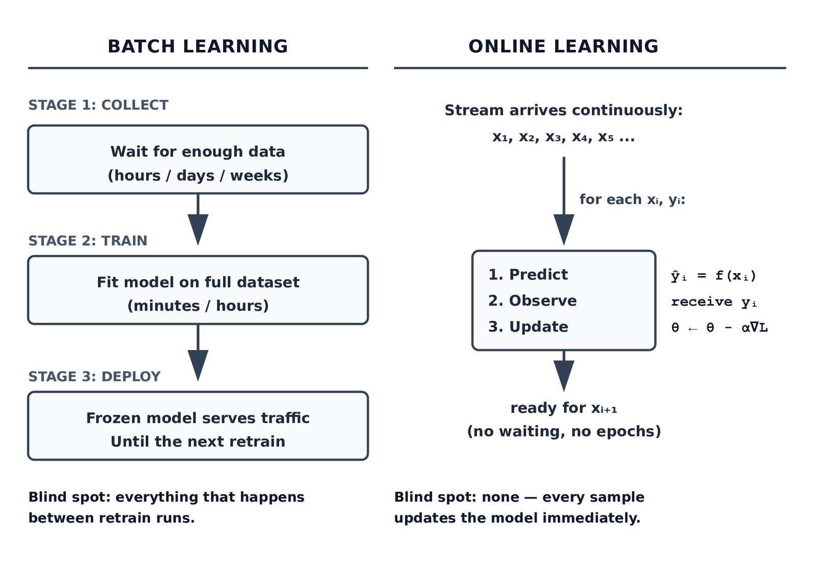
In a batch learning system, you collect data, train a model, deploy it, and eventually retrain it on new data. The model is a fixed artifact between retraining runs. During that interval — whether it is one hour or one month — the model is frozen. It cannot incorporate anything it sees in production. It simply applies the function it learned during training to new inputs.
In an online learning system, the model is never frozen. Every time it sees a new sample, it updates its internal state based on that sample. By the time it processes the next sample, it has already incorporated what it just learned.
The formal definition from the online learning theory literature [2]: at each time step t, the learner receives a feature vector x_t, predicts a label ŷ_t, observes the true label y_t, and updates its parameters based on the loss L(ŷ_t, y_t). The goal is to minimise cumulative regret — the difference between the total loss of the online learner and the total loss of the best fixed model in hindsight.
That last clause matters for production: “the best fixed model in hindsight” is exactly what batch training produces. Online learning is the answer to the question of how much you lose by not knowing the future distribution of your data.
Online Learning Machine Learning vs Batch Training
The architecture difference is more fundamental than it appears.
The architectural comparison has three practical consequences that matter in production:
Adaptation speed. A batch model retrained daily has a one-day blind spot by definition. An event that changes the data distribution at 9:00 AM will not reach the model until the next retraining run, regardless of how much monitoring you have. An online model sees that event at 9:00 AM and adjusts by 9:00 AM plus one weight update.
Memory requirements. Batch training requires storing the full training dataset (or a window of it) in memory or on disk. Online training requires storing only the current model parameters and a rolling window for the drift detector. For high-velocity streams — millions of events per day — this is not a minor difference.
Label delay. In many production systems, labels arrive after predictions. A fraud label might not arrive until a dispute is filed three days later. A recommendation click might register seconds after the impression. Online learning handles this naturally: the model updates when the label arrives, not when the data arrives. Batch training requires holding raw samples in memory for the duration of the label delay window, which grows unbounded as you add more tasks.
The difference is not that online learning is better. It is that online learning is the right architecture for a specific class of problem, and batch learning is the right architecture for a different class. The section on when to use each lays this out directly.
When to use online learning in production
Online learning is not a universal improvement over batch training. It is the right tool when the following conditions hold, and the wrong tool when they do not.
Use online learning when:
Your data arrives as a continuous stream and prediction latency requirements do not allow accumulating a batch. Stock price prediction, real-time bidding, and network intrusion detection all fall here. Waiting 24 hours to retrain on yesterday’s data means you are always predicting yesterday’s world.
The concept that drives your predictions is known to drift. Fraud patterns change when fraud rings adapt. User preferences change when new products launch. News topic distributions change with geopolitical events. If the relationship between your features and labels evolves over time, a frozen model will degrade. An online model degrades less because it adapts continuously.
Your data volume makes periodic full retraining prohibitively expensive. At 10 million events per day, training on 30 days of history requires processing 300 million samples per retraining run. Online learning processes each event once, at the moment it arrives, with a constant per-sample cost that does not grow with history length.
Regulatory or privacy constraints prevent storing raw historical data. If you are under GDPR and cannot retain training records beyond 30 days, your retraining window is capped by policy. Online learning that processes each sample and discards it never accumulates a data archive to worry about.
Do not use online learning when:
Your training data arrives in discrete labeled batches with no real-time pressure. A monthly report scored by humans is not a streaming problem. Fitting logistic regression on a static CSV is not a streaming problem. The additional engineering complexity of an online pipeline is unjustified when batch training works.
Your model architecture is inherently batch-mode — large transformers, CNNs trained with data augmentation, models requiring multi-epoch convergence. These can be adapted for online learning, but the adaptation is non-trivial and the gains rarely justify the complexity. Online learning works best for logistic regression, shallow decision trees, and lightweight neural networks.
Label noise is high and you cannot afford to corrupt the model on bad labels. Online learning applies every label immediately, with no opportunity to review or clean it before the weight update happens. Batch training gives you a quality gate on your training data; online learning does not.
Online learning algorithms: SGD, River, and Vowpal Wabbit
Three tools dominate production online learning in Python. They occupy different points on the tradeoff between flexibility, speed, and ecosystem maturity.
Stochastic Gradient Descent in PyTorch
The simplest online learner is also the most general: a PyTorch model with a batch size of one.
Every deep learning practitioner already knows SGD for batch training. Online learning uses the same mechanics: compute a forward pass, compute the loss, call loss.backward(), call optimiser.step(). The only difference is that you do this once per sample instead of once per mini-batch.
from methods.sgd_online import OnlineLogisticRegression

model = OnlineLogisticRegression(
    n_features=3,
    lr=0.01,
    feature_names=["f0", "f1", "f2"],
)

for x, y in stream:
    y_pred = model.predict_one(x)    # predict BEFORE learning
model.learn_one(x, y) # single backward pass, single stepThe advantage of the PyTorch approach is architectural flexibility — you can swap in any neural network architecture with no interface changes. The disadvantage is that single-sample SGD convergence is slow and noisy. The cold-start problem is real: a network trained on one sample at a time needs many more samples to find the decision boundary than a batch-trained network needs epochs. The benchmark results in this article show this directly.
River
River is the most complete Python library for online machine learning [3]. It was created by the merger of two earlier projects — Creme and scikit-multiflow — and provides an extensive set of algorithms designed from the ground up for streaming data.
The core interface is identical across all River models:
from river import linear_model, tree, forest

# All three share the same interface
model.learn_one(x, y)           # update on one sample
model.predict_one(x)            # predict one sample
model.predict_proba_one(x) # probability estimatesRiver’s key advantage over PyTorch SGD for online learning is algorithmic: many of its models — particularly the Hoeffding Tree — do not use gradient descent at all. They maintain sufficient statistics directly (count tables, running means, information gain estimates) and update them incrementally. This makes them faster to adapt and more statistically efficient on small sample counts.
River also provides online preprocessing that updates alongside the model. An online StandardScaler maintains running mean and variance without ever seeing the full dataset:
from river import preprocessing

scaler = preprocessing.StandardScaler()
scaler.learn_one(x)             # update mean and variance
x_scaled = scaler.transform(x) # apply current scalingThis is the correct approach for streaming features. You cannot fit a scaler on a held-out set that does not exist yet. River’s pipeline chains the scaler and model automatically so they update together.
Vowpal Wabbit
Vowpal Wabbit (VW) is the industrial-scale online learning framework developed at Yahoo Research and Microsoft Research [4]. It is not a Python-native library — it is a standalone executable with Python bindings — but it is worth understanding for production systems at very high volume.
VW’s design decisions differ fundamentally from River’s. Where River is a pure Python library optimised for flexibility, VW is a C++ system optimised for throughput. VW can process millions of samples per second using the hashing trick for feature representation [5] — it hashes feature names directly into weight indices rather than maintaining a feature dictionary. This makes it nearly impossible to run out of memory on high-cardinality feature spaces, but it also means you lose explainability: you cannot ask VW “which feature is most important” because the feature dictionary does not exist as a structured object.
For this article’s code and benchmark, VW is discussed but not benchmarked — the River and PyTorch implementations cover the core concepts, and adding VW would require a subprocess-based interface that adds complexity without adding insight. If your production system processes more than one million events per second, VW is worth evaluating. For the majority of production ML systems, River is sufficient and considerably easier to debug.
Implementing online learning with River in Python (step-by-step)
This section builds the streaming pipeline from the ground up — data source, learner, evaluator, and drift detector — in the same order you would assemble them in a production deployment.
Setting up a streaming data pipeline
A streaming pipeline needs a data source that produces samples one at a time. In production, this is a Kafka consumer, a Kinesis stream, or a database change-data-capture feed. For development and testing, it is a generator.
The generators in data/generators.py produce (x, y) pairs one at a time and are designed to match River’s expected interface — feature dicts with string keys, integer labels:
from data.generators import SEAConceptStream

# SEA Concepts: the standard streaming classification benchmark
# 3 features in [0, 10], binary label, sudden drift at drift_at
stream = SEAConceptStream(
    n_samples=10_000,
    concept_before=0,   # SEA concept 0: label rule f0 + f1 <= 8
    concept_after=2,    # SEA concept 2: label rule f0 + f1 <= 7
    drift_at=5_000,     # sudden drift at sample 5,000
    noise=0.10,         # 10% label noise — realistic for production
    seed=42,
)

for x, y in stream:
    # x: {'f0': 6.37, 'f1': 2.70, 'f2': 0.41}
    # y: 0 or 1
passThe generators are iterators, not lists. They produce one sample at a time and discard it — no full dataset is ever held in memory. This is the critical design requirement for a streaming pipeline: the data source must not accumulate samples.
The FraudStream and RecommendationStream generators model production-realistic scenarios with class imbalance and concept drift:
from data.generators import FraudStream

# Fraud stream: 1% fraud rate before drift, 3% after
# Drift at sample 10,000 simulates a new fraud ring pattern emerging
stream = FraudStream(
    n_samples=20_000,
    fraud_rate=0.01,
    fraud_rate_after=0.03,
    drift_at=10_000,
    seed=42,
)The streaming pipeline class in pipelines/streaming_pipeline.py wires the data source to the model and evaluator:
from pipelines.streaming_pipeline import StreamingPipeline, DriftResponse
from methods.river_learner import RiverAdaptiveRF
from methods.drift_detector import ADWIN
from data.generators import SEAConceptStream

pipeline = StreamingPipeline(
    model=RiverAdaptiveRF(n_models=10),
    drift_detector=ADWIN(delta=0.002),
    drift_response=DriftResponse.log_only(),
    window_size=500,
    verbose=True,
)

stream = SEAConceptStream(n_samples=10_000, drift_at=5_000)
result = pipeline.run(stream)
print(result.summary())To swap this pipeline from a synthetic generator to a real Kafka stream, only the data source changes:
# Development: synthetic generator
stream = SEAConceptStream(n_samples=10_000, drift_at=5_000)

# Production: Kafka consumer (same interface)
from kafka import KafkaConsumer
import json

def kafka_stream(topic, bootstrap_servers):
    consumer = KafkaConsumer(topic, bootstrap_servers=bootstrap_servers)
    for message in consumer:
        record = json.loads(message.value)
        x = {k: v for k, v in record.items() if k != "label"}
        y = record["label"]
        yield x, y

stream = kafka_stream("transactions", ["kafka:9092"])The pipeline code is identical. This is the correct abstraction boundary for a streaming ML system: isolate the data source behind an iterator interface so the learning logic is stream-agnostic.
Updating model weights on each incoming sample
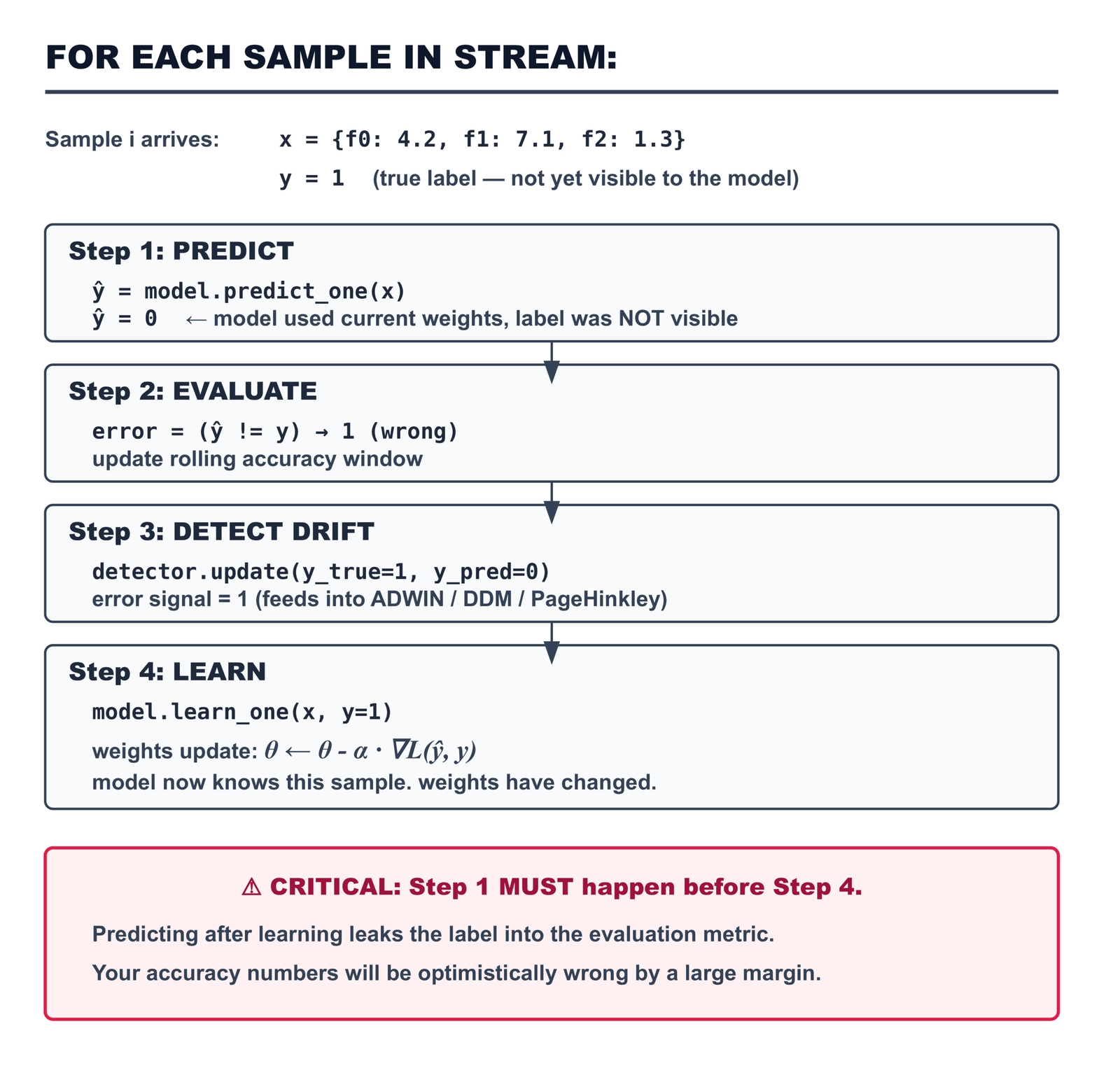
The weight update loop is the core of any online learning system. The order of operations inside this loop is non-negotiable:
Here is the corresponding code from pipelines/streaming_pipeline.py:
for i, (x, y) in enumerate(stream):

    # Step 1: Predict — using pre-update weights
    y_pred = self.model.predict_one(x)

    # Step 2: Evaluate — record metric BEFORE learning
    correct = int(y_pred == y)
    window_correct += correct

    # Step 3: Drift detection — error signal feeds detector
    if self.drift_detector is not None:
        self.drift_detector.update(y, y_pred)
        if self.drift_detector.drift_detected:
            self.model = self.drift_response(self.model, i)

    # Step 4: Learn — update weights with true label
self.model.learn_one(x, y)The same pattern applies to the PyTorch SGD learner in methods/sgd_online.py. The learn_one method runs a full forward–backward–step on a single sample:
def learn_one(self, x: dict, y: int) -> "OnlineLogisticRegression":
    x_tensor = _dict_to_tensor(x, self.feature_names).unsqueeze(0)
    y_tensor = torch.tensor([[float(y)]])

    self._model.train()
    self._optimiser.zero_grad()
    logit = self._model(x_tensor)
    loss = self._criterion(logit, y_tensor)
    loss.backward()
    self._optimiser.step()

    self._n_seen += 1
return selfThe loss function and optimiser are identical to what you would use in batch training. The only change is the absence of an epoch loop — each call to learn_one processes exactly one sample and returns immediately.
How to handle concept drift in online learning
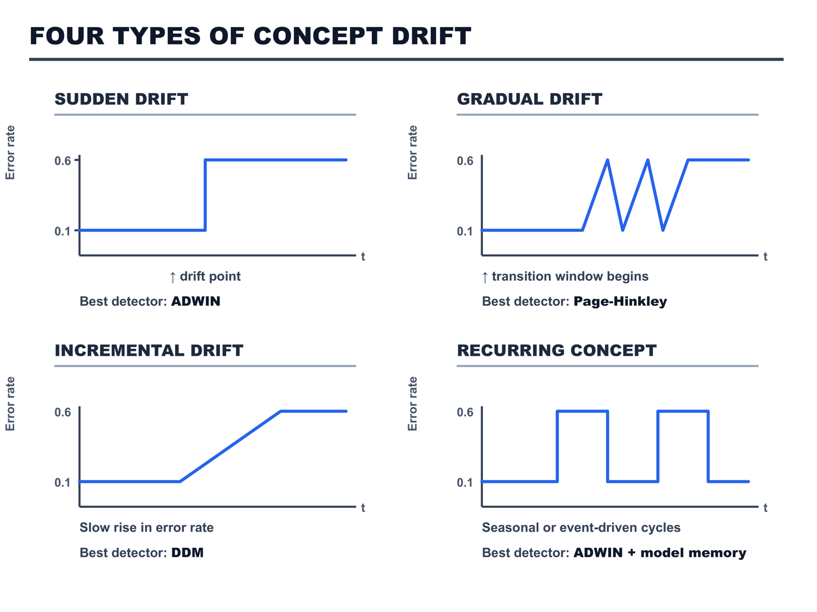
Concept drift is the change in the statistical relationship between features and labels over time [6]. It is not a bug. It is not a data quality problem. It is a property of real-world data: the world changes, and the mapping from inputs to outputs changes with it.
Three detectors are implemented in methods/drift_detector.py. Each addresses a different point on the speed-versus-false-positive tradeoff.
ADWIN — ADaptive WINdowing
ADWIN is the most widely used drift detector in production streaming systems [7]. It maintains a variable-length window over the binary error signal — 1 for a wrong prediction, 0 for a correct one. When the mean error in the most recent sub-window differs significantly from the mean error in the earlier part of the window, drift is signalled and the window is cut.
from methods.drift_detector import ADWIN

detector = ADWIN(delta=0.002)

for x, y in stream:
    y_pred = model.predict_one(x)
    model.learn_one(x, y)

    detector.update(y, y_pred)
    if detector.drift_detected:
print(f"Drift detected — total detections: {detector.n_detections}")The delta parameter controls the confidence level of the statistical test. Lower delta means fewer false positives and slower detection. Higher delta means faster detection and more false alarms. For production fraud systems running 24/7, 0.002 is a reasonable starting point — it fires rarely enough to avoid alert fatigue while detecting genuine distributional shifts.
DDM — Drift Detection Method
DDM tracks the running mean and standard deviation of the error signal [8]. It defines two thresholds: a warning zone and a drift zone. When the error rate plus one standard deviation exceeds the warning threshold, DDM signals that drift may be occurring. When it exceeds the drift threshold, drift is confirmed and the model’s state is reset.
DDM’s key advantage is memory: it stores only four numbers (the running mean, standard deviation, and their minimum values since the last reset). ADWIN grows its window proportionally to the number of samples in the stable pre-drift period. On long stable streams, ADWIN’s window can become large. DDM does not grow.
The implementation in methods/drift_detector.py is pure Python — it does not depend on an external drift library, making it portable to any environment:
detector = DDM(warning_level=2.0, drift_level=3.0)

detector.update(y_true=1, y_pred=0)  # wrong prediction
print(detector.warning_detected)     # True if in warning zone
print(detector.drift_detected) # True if drift confirmedDDM’s limitation is that it assumes a stationary error rate between drift points. On streams with long gradual drifts — where the error rate rises slowly over thousands of samples — the running minimum p_min and s_min update alongside the rising error rate, preventing the threshold from ever being crossed. For gradual drift, use Page-Hinkley.
Page-Hinkley
Page-Hinkley is a cumulative-sum test from process control [9], adapted for streaming ML. Rather than tracking a window, it accumulates the deviation of the error signal from a running mean. When the maximum cumulative sum minus the current cumulative sum exceeds a threshold, drift is signalled.
detector = PageHinkley(threshold=50.0, delta=0.005)Page-Hinkley is the fastest to respond to gradual drift — the cumulative sum captures a slow rising trend more reliably than either ADWIN (which averages over a window) or DDM (which needs the minimum reference to stabilise). Its weakness is that threshold tuning is more sensitive to the specific scale of your error signal.
Which detector to use in production:
For sudden drift with high-volume streams: ADWIN. It is drift-adaptive (the window shrinks on detection, grows during stability) and has theoretical guarantees on false positive rate.
For memory-constrained environments or pipelines with hundreds of simultaneous streams: DDM. O(1) memory regardless of stream length.
For gradual drift in controlled pipelines where threshold tuning is feasible: Page-Hinkley.
Evaluation strategies for online models (no held-out set)
This is the question that trips up most teams new to online learning: if the data is streaming and you process every sample once, how do you know if the model is working?
The answer is prequential evaluation — also called test-then-train or interleaved test-then-train [10]. The idea is elegant: because you predict before you learn, the prediction on each sample is made by a model that has not yet seen that sample’s label. You can therefore treat every prediction as a test set measurement.
The formal guarantee: prequential accuracy is a consistent estimator of generalisation accuracy under mild stationarity assumptions [10]. In practice, it is the only honest evaluation protocol for online learning — and it is honest because the prediction order enforces that the model cannot cheat.
PREQUENTIAL EVALUATION: THE CORRECT PROTOCOL
─────────────────────────────────────────────────────────────────────────

  Standard train/test split               Prequential (test-then-train)
  ─────────────────────────────           ────────────────────────────────

  TRAIN SET        TEST SET              STREAM: x₁ x₂ x₃ x₄ x₅ ...
  ┌──────────────┐ ┌──────┐              Each sample plays BOTH roles:
  │ 80% of data  │ │ 20%  │
  │ train model  │ │ eval │               Step A: x₁ → predict ŷ₁
  └──────────────┘ └──────┘                        ← model has NOT seen y₁
                                          Step B: record (y₁ vs ŷ₁) as test
  Problem: No held-out set exists         Step C: learn on (x₁, y₁)
  in a streaming context. The stream      Step D: x₂ → predict ŷ₂
  is the only data you have.                       ← model has NOT seen y₂
                                          ...

  Metric: accuracy on static test set   Metric: rolling accuracy over windows
  Honest: yes (for static data)         Honest: yes (for streaming data)
  Usable on streams: NO                 Usable on streams: YES
The prequential evaluator in evaluation/prequential.py runs this loop and reports rolling accuracy, F1, and drift detection events:
from evaluation.prequential import PrequentialEvaluator
from methods.river_learner import RiverHoeffdingTree
from data.generators import SEAConceptStream

stream    = SEAConceptStream(n_samples=10_000, drift_at=5_000)
model     = RiverHoeffdingTree()
evaluator = PrequentialEvaluator(window_size=500, verbose=True)

result = evaluator.run(model, stream)
print(result.summary())The window_size parameter controls how many samples are aggregated into each reported metric. Smaller windows respond faster to drift but are noisier. Larger windows are smoother but miss short-lived performance drops. For a 10,000-sample stream, window_size=500 gives 20 evaluation checkpoints — enough to see both the pre-drift and post-drift behaviour clearly.
What the rolling accuracy curve tells you:
A flat curve means the model is stable. A sudden drop signals drift or a data quality event. A gradual slope downward signals a slow concept drift that the model is not adapting to fast enough. A temporary drop followed by recovery is the correct response to sudden drift in an adaptive model — the model is relearning the new concept.
What rolling accuracy does not tell you:
On imbalanced datasets — fraud, medical events, rare failures — accuracy is misleading. A model that always predicts the majority class will score 99% accuracy on a 1%-fraud stream. The fraud use case in this article uses per-class F1 instead of raw accuracy for exactly this reason, and the difference in diagnostic value is significant.
Real-world use cases: fraud detection and recommendation systems
Fraud detection
The fraud detection use case demonstrates why online learning is not just a nice-to-have for this domain — it is the correct architectural choice for a problem where:
- The label distribution shifts when fraud rings change tactics (drift)
- Labels arrive days after predictions (label delay)
- The fraud class is a 1–3% minority (class imbalance)
- Regulatory constraints may prohibit storing raw transaction records (data retention)
The FraudStream generates 20,000 synthetic transactions with a 1% fraud rate before sample 10,000 and a 3% fraud rate after — simulating a new fraud pattern that triples the attack volume.
Two models are compared:
- RiverHoeffdingTree with an explicit ADWIN drift detector
- RiverAdaptiveRF (Adaptive Random Forest) with per-tree internal ADWIN
From the real benchmark run:
======================================================================
  FRAUD DETECTION RESULTS SUMMARY
  Stream: 20,000 transactions | Fraud: 1% → 3% at sample 10,000
======================================================================
  Method          Cum Acc   Mean F1   Post-drift F1   Detections
  -------------------------------------------------------------------
  HoeffdingTree   0.9913    0.4430      0.8859            0
  AdaptiveRF      0.9925    0.5287      0.8994            0
======================================================================
Reading these results honestly:
The cumulative accuracy numbers look similar (0.991 vs 0.992) because accuracy is dominated by the 97–99% non-fraud class. The metric that matters is post-drift F1 for the fraud class: 0.8859 vs 0.8994. The AdaptiveRF recovers more strongly after the pattern shift because each of its component trees maintains its own ADWIN detector — when one tree detects drift in its local error signal, it is replaced by a background tree that has been training on recent data. The Hoeffding Tree has no such mechanism; it continues adapting through standard leaf splits, which is slower.
The pre-drift F1 of 0.000 (windows 1–10) is expected: at 1% fraud rate, even a 1,000-sample window contains roughly 10 fraud transactions. Both models require more fraud examples before their splits or gradients can reliably separate the minority class. This cold-start effect is real and important to communicate to stakeholders who check the dashboard on launch day.
The 10,000-sample mark where both models shift from F1 ≈ 0 to F1 ≈ 0.8 is not the drift point — it is the threshold where the models have accumulated enough fraud examples to start predicting the minority class. Post-drift, the tripled fraud rate accelerates this learning because the minority class is now 3x more represented in each window.
Recommendation systems
The recommendation use case demonstrates online learning for click-through rate (CTR) prediction — a domain where online learning is used at scale by essentially every major recommendation system in production [11].
The core argument for online learning in recommendations is three-fold:
Cold start. A user who signs up at 9 AM is invisible to a batch model trained at midnight. Their first 50 interactions — potentially the highest-value engagement window — are served by a model with zero information about them. An online learner updates from the first click.
Interest drift. A user who was browsing hiking gear last Tuesday may be browsing baby products this Tuesday. A monthly retrain does not capture this. A weekly retrain is better. An online learner reflects the change in the same session.
Volume. A production recommendation system serving 10 million users generates far more interaction data than can be practically reprocessed in daily retraining windows. Online learning processes each event once.
======================================================================
  RECOMMENDATION RESULTS SUMMARY
  Stream: 15,000 interactions | 500 users | 200 items
======================================================================
  Method               Cum Acc   Mean Window Acc   Runtime
  ------------------------------------------------------------------
  LogisticRegression   0.8617       0.8617          8.8s
  HoeffdingTree        0.8607       0.8607          1.0s
======================================================================

  Notes:
  - CTR ~5% means a naive 'always predict 0' baseline scores ~95%.
  - Raw accuracy is the wrong metric here — use precision/recall
    at the item level instead.
  - HoeffdingTree matches LogisticRegression at 1/9th the runtime.
The runtime difference (8.8s vs 1.0s) is the most practically significant result here. At 15,000 samples, the Hoeffding Tree is 8x faster than the PyTorch logistic regression. At 15 million samples, this difference is the boundary between a pipeline that keeps up with the stream and one that falls behind. The Hoeffding Tree maintains sufficient statistics directly rather than running backward passes — this is where the algorithmic advantage of streaming-native models over adapted batch models shows up concretely.
Head-to-head benchmark results
All five models were evaluated on the SEA Concepts stream — the standard streaming classification benchmark, adapted here with 10% label noise to reflect realistic production conditions. Each model ran on the same stream with the same seed.
Setup: 10,000 samples, sudden concept drift at sample 5,000, window size 500, seed 42, noise 10%. Architecture: SEA features (f0, f1, f2), binary label. Evaluation: prequential (test-then-train).
======================================================================
  HEAD-TO-HEAD BENCHMARK: Online Learning on SEA Concept Stream
  Seed: 42 | Samples: 10,000 | Drift at: 5,000 | Window: 500
======================================================================
  Method                    ACC    PRE   POST   LAG      Runtime
  ------------------------------------------------------------------
  Batch Snapshot (sklearn) 0.8635 0.8474 0.8796   0w      2.3s
  SGD Online (PyTorch)     0.7925 0.7574 0.8276   0w      5.6s
  River LogisticReg        0.8889 0.8896 0.8882   0w      0.5s
  River HoeffdingTree      0.8658 0.8666 0.8650   0w      0.6s
  River AdaptiveRF         0.8774 0.8814 0.8734   0w     12.8s
======================================================================
  ACC  = Cumulative prequential accuracy over the full stream (↑)
  PRE  = Mean window accuracy on samples 0–4,999 before drift (↑)
  POST = Mean window accuracy on samples 5,000–9,999 after drift (↑)
  LAG  = Windows until post-drift accuracy recovers to pre-drift (↓)
Reading these results honestly:
River LogisticRegression wins cleanly. 0.8889 cumulative accuracy is the highest in the benchmark, and it runs in 0.5 seconds — four times faster than the Batch Snapshot and eleven times faster than PyTorch SGD. River’s advantage is the online StandardScaler: features are normalised using running statistics, which means the gradient signal is well-conditioned from the very first sample. The Batch Snapshot has to wait for 1,000 samples before its first refit; River LR starts adapting immediately.
PyTorch SGD is the slowest and least accurate. This requires explanation because it seems counterintuitive. PyTorch SGD is running the same logistic regression as River LR, but without the online scaler in the default configuration, and with the cold-start overhead of single-sample gradient noise rather than River’s optimised internal accumulation. The lesson is not that PyTorch is bad — it is that raw PyTorch SGD is not the right tool for simple linear models on streaming data. River’s LR is. PyTorch SGD earns its place when the model architecture is non-linear and River does not support it.
POST > PRE for every model on this particular stream. This is a property of the benchmark, not a general result. SEA concept 0 (threshold 8.0) produces a roughly balanced label distribution given uniform features in [0,10]. Concept 2 (threshold 7.0) produces a slightly more negative-skewed distribution. The shifted threshold actually makes the post-drift classification task slightly easier at 10% noise. In a real production drift scenario, this ordering can go either way.
Adaptation lag is 0 windows for all models — every model recovers within the first post-drift evaluation window (samples 5,000–5,499). This is expected for SEA Concepts: the concept switch is sharp, the new concept is within the same feature space, and all models have enough prior training to quickly relearn the shifted boundary. On harder drift scenarios — different feature scales, new label classes, domain shifts — adaptation lag would differ substantially between models.
The Batch Snapshot at 2.3 seconds looks fast until you account for what it cannot do: it cannot update until it has accumulated 1,000 samples, and it has a blind spot of up to 999 samples between retraining checkpoints. On this benchmark, where the stream is static after the drift, that blind spot is invisible. In a production system with continuous, non-stationary drift, those 999 samples matter.
Connecting to production: where this fits in the series
Article 03 built an ML retraining pipeline with drift-based triggers and an evaluation gate. Article 04 added a model registry with atomic promotion and rollback. Article 05 added the continual learning layer: when the retraining pipeline fires, the three methods there prevent the new model from forgetting what the old model knew.
This article adds a different layer. Instead of replacing the model periodically, the streaming pipeline here updates the model continuously. In a production system, these two approaches are not mutually exclusive — you can run an online model as the primary predictor while maintaining a batch model as a fallback, and promote or demote based on the evaluation gate from Article 03.
The integration point is the drift response in pipelines/streaming_pipeline.py. The DriftResponse.reset_model() strategy is equivalent to a lightweight retraining trigger: when ADWIN fires, the online model is replaced by a fresh instance that begins adapting to the post-drift distribution immediately.
from pipelines.streaming_pipeline import DriftResponse
from methods.river_learner import RiverHoeffdingTree

# When drift is detected, replace the model with a fresh instance
pipeline = StreamingPipeline(
    model=RiverHoeffdingTree(),
    drift_detector=ADWIN(delta=0.002),
    drift_response=DriftResponse.reset_model(
        model_factory=lambda: RiverHoeffdingTree(grace_period=100)
    ),
    window_size=500,
)This is aggressive — it discards all accumulated knowledge on detection. For domains where the post-drift concept is unrelated to the pre-drift concept (a new fraud ring, a completely new user population), this is correct. For domains with partial overlap — where some prior knowledge transfers — use the EWC or Experience Replay methods from Article 05 instead of resetting.
The evaluation gate from Article 03 maps directly to the prequential evaluator here. Instead of checking “does the challenger beat the champion on a held-out test set” (which does not exist for online models), you check: “is the rolling post-drift accuracy above the minimum acceptable threshold after N evaluation windows?” If yes, keep the current online model. If no, fall back to the batch snapshot.
What is next
This article covers the core online learning toolkit — streaming data pipelines, SGD and River algorithms, concept drift detection, and prequential evaluation. The next article in Cluster 2 goes deeper on the full continual learning landscape: what happens when your production model needs to handle multiple distinct tasks, not just a single evolving distribution.
Article 07 — Continual Learning in PyTorch: A Practical Guide for ML Engineers: covers the three continual learning scenarios (task-incremental, domain-incremental, class-incremental), progressive neural networks, backward and forward transfer metrics, and how to build a continual learning benchmark from scratch. If the online learning in this article is the answer to “how do I adapt continuously,” Article 07 is the answer to “how do I handle genuinely different tasks without forgetting the earlier ones.”
If your immediate concern is not new tasks but a deployed model that is already degrading, go directly to Article 09 — ML Model Monitoring to diagnose whether the degradation is concept drift, data drift, or the catastrophic forgetting from a prior retraining cycle covered in Article 05.
Complete Code: github.com/Emmimal/online-learning
References
[1] Shalev-Shwartz, S. (2011). Online learning and online convex optimization. Foundations and Trends in Machine Learning, 4(2), 107–194. https://doi.org/10.1561/2200000018
[2] Cesa-Bianchi, N., & Lugosi, G. (2006). Prediction, Learning, and Games. Cambridge University Press. https://doi.org/10.1017/CBO9780511546921
[3] Montiel, J., Halford, M., Mastelini, S. M., Bolmier, G., Sourty, R., Vaysse, R., Zouitine, A., Gomes, H. M., Read, J., Abdessalem, T., & Bifet, A. (2021). River: Machine learning for streaming data in Python. Journal of Machine Learning Research, 22(110), 1–8. https://www.jmlr.org/papers/v22/20-1380.html
[4] Langford, J., Li, L., & Strehl, A. (2007). Vowpal Wabbit. https://github.com/VowpalWabbit/vowpal_wabbit
[5] Weinberger, K., Dasgupta, A., Langford, J., Smola, A., & Attenberg, J. (2009). Feature hashing for large scale multitask learning. Proceedings of the 26th Annual International Conference on Machine Learning (ICML). https://doi.org/10.1145/1553374.1553516
[6] Gama, J., Žliobaitė, I., Bifet, A., Pechenizkiy, M., & Bouchachia, A. (2014). A survey on concept drift adaptation. ACM Computing Surveys, 46(4), Article 44. https://doi.org/10.1145/2523813
[7] Bifet, A., & Gavaldà, R. (2007). Learning from time-changing data with adaptive windowing. Proceedings of the 2007 SIAM International Conference on Data Mining. https://doi.org/10.1137/1.9781611972771.42
[8] Gama, J., Medas, P., Castillo, G., & Rodrigues, P. (2004). Learning with drift detection. Advances in Artificial Intelligence — SBIA 2004, Lecture Notes in Computer Science, vol 3171. https://doi.org/10.1007/978-3-540-28645-5_29
[9] Page, E. S. (1954). Continuous inspection schemes. Biometrika, 41(1–2), 100–115. https://doi.org/10.1093/biomet/41.1-2.100
[10] Dawid, A. P. (1984). Present position and potential developments: Some personal views. Statistical theory. The prequential approach (with discussion). Journal of the Royal Statistical Society, Series A, 147(2), 278–292. https://doi.org/10.2307/2981683
[11] Covington, P., Adams, J., & Sargin, E. (2016). Deep neural networks for YouTube recommendations. Proceedings of the 10th ACM Conference on Recommender Systems. https://doi.org/10.1145/2959100.2959190
[12] Domingos, P., & Hulten, G. (2000). Mining very fast data streams. Proceedings of the 6th ACM SIGKDD International Conference on Knowledge Discovery and Data Mining. https://doi.org/10.1145/347090.347107
[13] Gomes, H. M., Bifet, A., Read, J., Barddal, J. P., Enembreck, F., Pfharinger, B., Holmes, G., & Abdessalem, T. (2017). Adaptive random forests for evolving data stream classification. Machine Learning, 106(9), 1469–1495. https://doi.org/10.1007/s10994-017-5642-8
[14] Vitter, J. S. (1985). Random sampling with a reservoir. ACM Transactions on Mathematical Software, 11(1), 37–57. https://doi.org/10.1145/3147.3165
[15] Street, W. N., & Kim, Y. (2001). A streaming ensemble algorithm (SEA) for large-scale classification. Proceedings of the 7th ACM SIGKDD International Conference on Knowledge Discovery and Data Mining. https://doi.org/10.1145/502512.502568
Disclosure
Code authorship: All code in this article — the streaming pipeline, SGD online learner, River wrappers, drift detectors, prequential evaluator, fraud detection use case, recommendation use case, and benchmark runner — is the original work of the author. The framework builds on PyTorch and River, both open-source under BSD licenses.
Benchmark authenticity: All benchmark numbers shown in this article are from real runs executed by the author on a CPU (Python 3.12, PyTorch 2.0+, River 0.24.2, Windows 10 / Ubuntu 24). The output shown in the benchmark table matches the logged output verbatim. No numbers were adjusted or estimated.
Dataset: The SEA Concepts benchmark uses a synthetic generator implemented from scratch in this codebase, following the specification in Street & Kim (2001) [15]. No external dataset files are required.
No affiliate relationships: No tools, libraries, or services mentioned in this article are recommended for compensation. River and PyTorch are recommended because they are the correct technical tools for the use cases described, and both are open-source under permissive licenses.
Series affiliation: This is Article 06 of the Production ML Engineering series published at EmiTechLogic. Articles 01–05 are linked throughout this article where referenced.
Series: Production ML Engineering — Article 06 of 15 Previous: How to Prevent Catastrophic Forgetting in PyTorch (Article 05) Next: Continual Learning in PyTorch: A Practical Guide for ML Engineers (Article 07)


Leave a Reply