
")
How to Prevent Catastrophic Forgetting in PyTorch (Complete Guide)
Catastrophic forgetting in PyTorch is one of the most common problems when training models on sequential tasks. As new data is introduced, models often overwrite previously learned knowledge, leading to sudden performance drops.
Series: Production ML Engineering — Article 05 of 15 (Cluster 2: Continual Learning)
Before you read this: This article is part of a 15-part series on building production-grade ML systems. If you have not read the series hub yet, start with the Production ML Engineering guide — it maps out the five pillars every production system rests on and explains where this article fits. Articles 02–04 covered deployment, retraining pipelines, and model versioning. This article opens Cluster 2 by addressing what happens when retraining destroys what the model already knew.
Six months after a model ships, you retrain it on fresh data. Evaluation metrics look fine. You promote it through the registry, the CI/CD pipeline passes, the smoke test clears. Everything looks clean.
Two days later, a stakeholder flags that a segment of predictions that used to work well is now completely broken. You dig in. The model has lost its memory of an entire data distribution it was trained on months ago. Not because of drift. Not because of a data quality issue. Because you retrained it, and it forgot.
This is catastrophic forgetting. And it is not a fringe concern — it is one of the most underestimated failure modes in production ML systems that undergo regular retraining.
This article documents three strategies to prevent it — Elastic Weight Consolidation (EWC), Experience Replay, and PackNet — with complete PyTorch implementations, a head-to-head benchmark on Split-MNIST, and an honest account of when each method stops working. Everything is code-first. All benchmark numbers are from real runs on the architecture described in this series.
Complete Code: github.com/Emmimal/catastrophic-forgetting
What is catastrophic forgetting in PyTorch?
Catastrophic forgetting — also called catastrophic interference — is the tendency of artificial neural networks to abruptly lose previously learned information upon learning new information [1].
Simple definition: when you fine-tune a neural network on new data, it overwrites the weights that encoded old knowledge. Old task accuracy collapses. The network did not get worse at the old task because the world changed — it got worse because gradient updates for the new task destroyed the parameters that made the old task work.
McCloskey and Cohen first documented this systematically in 1989 using connectionist models [2], and for decades it was treated as a research curiosity rather than a production concern. That has changed. As ML teams began retraining models on rolling data windows — fraud detection models refreshed monthly, recommendation systems updated weekly, NLP classifiers fine-tuned on new domains — the problem became unavoidable.
The reason it is especially dangerous in production is that it is invisible at the moment it happens. The new model passes its evaluation gate on the new data distribution. It passes the smoke test. The monitoring dashboard shows healthy prediction volume. The forgetting only surfaces when someone checks a segment of the prediction space that was not covered by the recent evaluation data — which could be days later, or never, if nobody is checking that segment.
Why catastrophic forgetting in PyTorch happens
Understanding why forgetting happens is necessary for understanding why the three prevention strategies work. The mechanism is gradient interference.
When a network trains on Task A, gradient descent finds a region of the parameter space where the loss for Task A is minimised. Call this region θ*_A. When you then train on Task B, gradient descent moves the parameters toward a region where Task B’s loss is minimised — call it θ*_B. The problem is that these two regions are almost never the same point in parameter space, and the path from θ*_A toward θ*_B passes through regions where Task A’s loss is high.
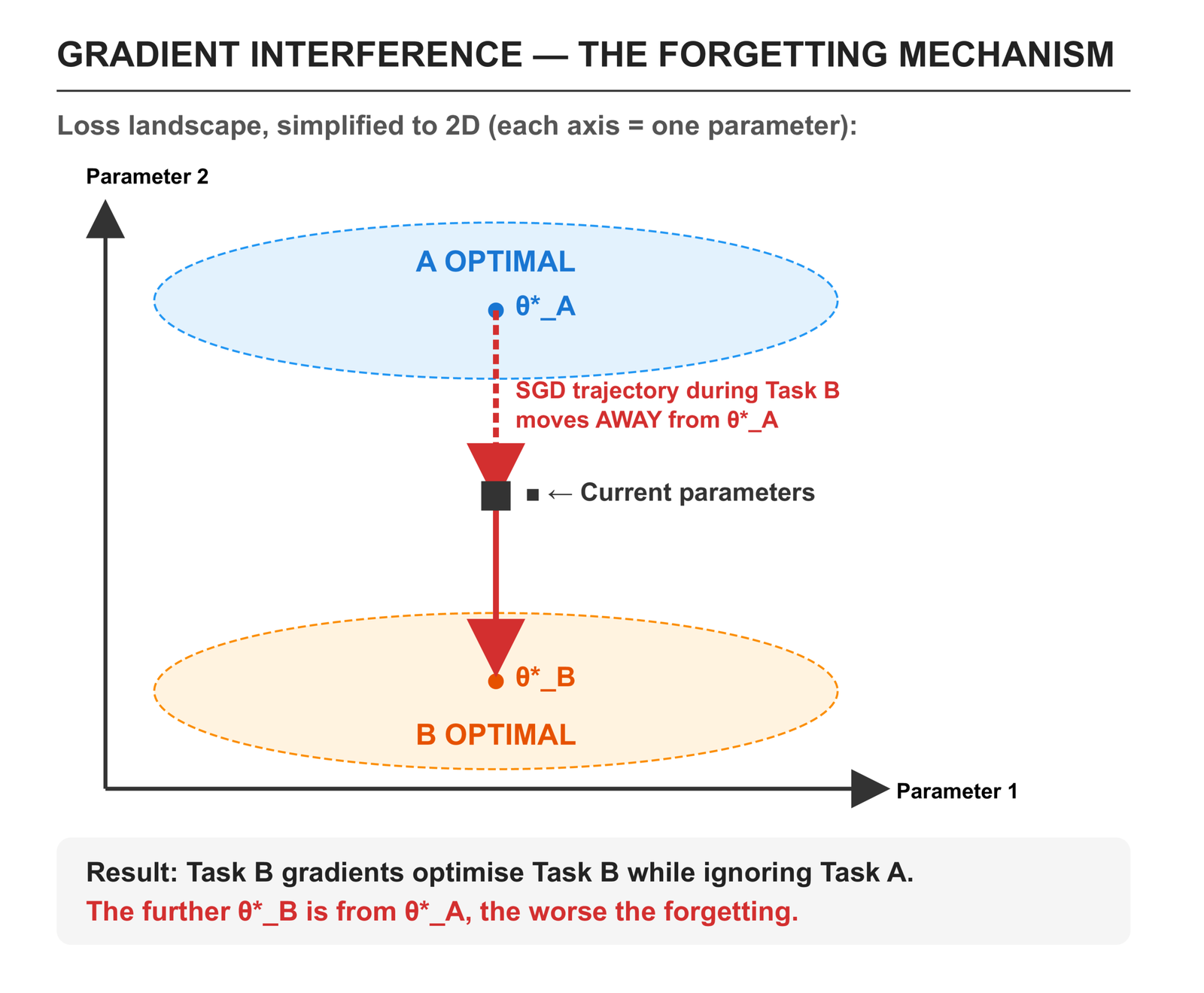
There is no malfunction here. The network is doing exactly what it was asked to do: minimise the loss on the current task. It has no memory that Task A ever existed. The gradients have no mechanism to preserve parameters that were useful for a task no longer present in the training data.
Three classes of solutions have emerged in the continual learning literature [3]:
Regularisation-based methods add a penalty to the loss function that resists changes to parameters important for prior tasks. EWC is the most cited example [4].
Replay-based methods maintain a buffer of old training examples and mix them into new training batches, keeping the old task present in the gradient signal [5].
Architecture-based methods partition the network so that different parameter subsets are dedicated to different tasks. PackNet is the canonical implementation [6].
Each addresses the gradient interference problem differently, and each has failure modes the others do not. All three are benchmarked in this article against the same model on the same data so the trade-offs are visible rather than theoretical.
How to prevent catastrophic forgetting in PyTorch using Elastic Weight Consolidation (EWC)
Elastic Weight Consolidation was introduced by Kirkpatrick et al. at DeepMind in 2017 [4]. It is the most widely cited regularisation-based approach to catastrophic forgetting, and the one that most production teams reach for first.
How EWC Works: Fisher Information Matrix Explained
The core idea is to identify which weights matter most for the task you have already trained, and then make those weights expensive to change.
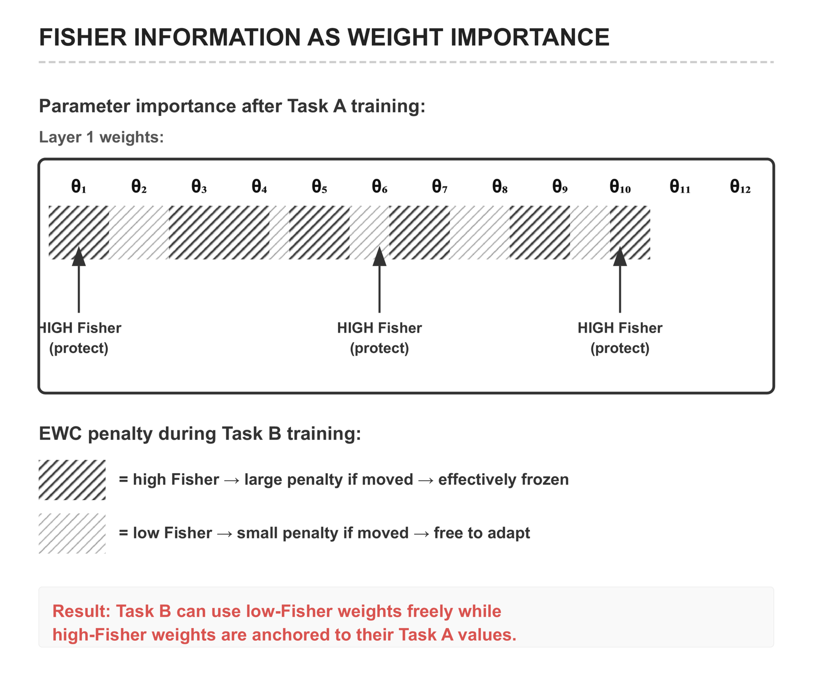
After training Task A, EWC estimates the importance of each parameter using the diagonal of the Fisher Information Matrix (FIM). The Fisher diagonal F_i for parameter θ_i measures how much the model’s output distribution changes when θ_i changes — parameters with high Fisher values are critical to the model’s predictions; changing them substantially will hurt performance on Task A.
The Fisher diagonal is estimated using the empirical Fisher approximation: for each training sample, compute the gradient of the log-probability of the model’s own predicted label with respect to each parameter, then square and average these gradients:
F_i ≈ (1/N) Σ_n [ ∂/∂θ_i log P(ŷ_n | x_n) ]²High F_i = large gradient variance = parameter matters for this task. Low F_i = small gradient variance = parameter can change without hurting the task.
Once the Fisher diagonal is estimated, EWC adds a regularisation penalty when training the next task:
L_total = L_task_B + (λ/2) Σ_i F_i · (θ_i − θ*_i)²where θ*_i is the parameter value after training Task A (the anchor), and λ controls the strength of the resistance. The penalty is zero when parameters stay at their Task A values and grows quadratically as they deviate.
Tuning λ — the forgetting/plasticity trade-off:
This is a genuine tension with no universal answer.
- λ too high → the model resists learning Task B (high-Fisher weights dominate, blocking gradient flow toward the Task B optimum)
- λ too low → the model overwrites Task A knowledge (penalty is too weak to meaningfully constrain weight movement)
- λ right → Task B learning converges while prior task accuracy is preserved within acceptable bounds
Tune λ on a held-out validation set that contains examples from both the old task and the new task. A dataset with only new-task examples will make any λ above zero look harmful. The typical range is 0.1–10.0; start at 0.4 and search.
EWC Implementation in PyTorch (Full Code)
The standalone loss function, as it appears in the article’s code:
def ewc_loss(model, original_params, fisher_diag, criterion,
             outputs, labels, lambda_ewc=0.4):
    """
    Combines task loss with EWC regularisation.

    lambda_ewc controls a genuine tension:
      - Too high → model resists learning new patterns (underfits new distribution)
      - Too low  → model overwrites old knowledge (catastrophic forgetting)
    Tune this on a held-out evaluation set that includes both old and new examples.
    """
    task_loss = criterion(outputs, labels)

    ewc_penalty = 0
    for name, param in model.named_parameters():
        fisher    = fisher_diag[name]
        old_param = original_params[name]
        ewc_penalty += (fisher * (param - old_param) ** 2).sum()

return task_loss + (lambda_ewc / 2) * ewc_penaltyThe production EWC trainer wraps this in a class that handles Fisher estimation and anchor snapshotting. The Fisher diagonal is estimated over n_fisher_samples training examples using per-sample backward passes:
# methods/ewc.py — EWC._estimate_fisher()

fisher: Dict[str, torch.Tensor] = {
    name: torch.zeros_like(param)
    for name, param in self.model.named_parameters()
    if param.requires_grad
}

for x, y in train_loader:
    if n_samples >= self.n_fisher_samples:
        break

    for i in range(x.size(0)):
        xi = x[i : i + 1]
        self.model.zero_grad()

        logits    = self.model(xi, task_id=task_id)
        log_probs = torch.log_softmax(logits, dim=1)
        predicted = logits.argmax(dim=1)

        # Empirical Fisher: gradient of log P(ŷ | x)
        loss = -log_probs[0, predicted[0]]
        loss.backward()

        for name, param in self.model.named_parameters():
            if param.grad is not None:
                fisher[name] += param.grad.data ** 2

        n_samples += 1

# Normalise
for name in fisher:
fisher[name] /= n_samplesUsing the EWC trainer:
from methods.ewc import EWC
from models.mlp import MultiHeadMLP

model = MultiHeadMLP(input_dim=784, hidden_dims=[256, 256], head_output_dim=2)
model.add_task_head()   # Task 0
model.add_task_head()   # Task 1

trainer = EWC(
    model=model,
    lambda_ewc=0.4,
    n_fisher_samples=200,
    multi_head=True,
)

# Task 0 — no EWC penalty yet (no prior tasks)
trainer.train_task(0, train_loader_task0, epochs=5)

# Consolidate: compute Fisher diagonal + snapshot anchor weights
trainer.consolidate(0, train_loader_task0)

# Task 1 — EWC penalty now protects Task 0's high-Fisher weights
trainer.train_task(1, train_loader_task1, epochs=5)

acc_task0 = trainer.evaluate(0, test_loader_task0)
acc_task1 = trainer.evaluate(1, test_loader_task1)Online EWC for multiple tasks: When more than one prior task exists, this implementation accumulates Fisher diagonals rather than storing separate FIM + anchor sets per task. The accumulated Fisher is the sum over all prior tasks. This is the online EWC variant [7] — computationally cheaper and equivalent in practice for moderate numbers of tasks.
How to prevent catastrophic forgetting in PyTorch with Experience Replay
Experience Replay is the oldest and conceptually simplest approach to catastrophic forgetting [5]. After training on Task A, store a small random subset of Task A’s training examples in a fixed-size buffer. When training on Task B, interleave old examples from the buffer with new Task B examples in each mini-batch.
The mechanism is direct: keep the old task present in the gradient signal by continuing to show the model examples from it. The network cannot forget what it keeps being trained on.
Reservoir sampling: The buffer uses Vitter’s reservoir sampling algorithm [8] to maintain a uniform random sample of all examples seen since initialisation. Each incoming example replaces a buffer slot with probability buffer_size / n_seen. This is critical — naive approaches like keeping the first N examples or keeping the last N examples produce biased buffers that over-represent certain tasks. Reservoir sampling guarantees uniformity without knowing the stream length in advance.
def add_batch(self, x, y, task_id):
    """Reservoir sampling — uniform sample of all data seen so far."""
    for i in range(x.size(0)):
        self._n_seen += 1

        if len(self._buffer_x) < self.capacity:
            # Buffer not full — always add
            self._buffer_x.append(x[i])
            self._buffer_y.append(y[i])
            self._buffer_task_ids.append(task_id)
        else:
            # Replace with probability capacity / n_seen
            j = self._rng.randint(0, self._n_seen - 1)
            if j < self.capacity:
                self._buffer_x[j] = x[i]
                self._buffer_y[j] = y[i]
self._buffer_task_ids[j] = task_idUsing the Experience Replay trainer:
from methods.experience_replay import ExperienceReplay

trainer = ExperienceReplay(
    model=model,
    buffer_size=500,      # 500 examples across all tasks
    replay_ratio=0.5,     # 50% of each mini-batch from the buffer
    multi_head=True,
)

# Buffer fills during Task 0 training
trainer.train_task(0, train_loader_task0, epochs=5)

# During Task 1, old Task 0 examples are mixed into every batch
trainer.train_task(1, train_loader_task1, epochs=5)

print(trainer.buffer_stats())
# {'size': 500, 'capacity': 500, 'task_distribution': {0: 268, 1: 232}}The task distribution after Task 1 shows reservoir sampling at work: Task 0 still owns roughly half the buffer even after 500 Task 1 examples have passed through. If you had used a naive FIFO buffer, Task 0 would be mostly evicted by now.
The replay_ratio hyperparameter controls the fraction of each mini-batch from the buffer. A ratio of 0.5 means each gradient step is computed on 50% new examples and 50% old examples. Too low and the gradient signal is dominated by the new task. Too high and convergence on the new task slows unnecessarily. For Split-MNIST with 5 tasks, 0.3–0.5 works well.
How to prevent catastrophic forgetting in PyTorch using PackNet
PackNet, introduced by Mallya and Lazebnik at CVPR 2018 [6], takes a structurally different approach: rather than approximately preventing forgetting through regularisation or replay, it eliminates forgetting by design.
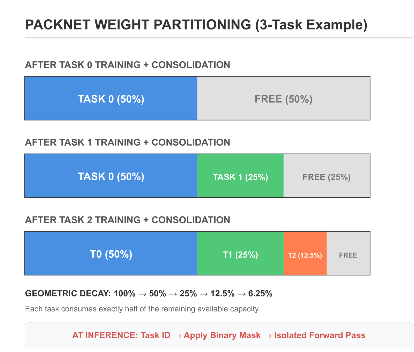
The mechanism is iterative pruning and freezing. After training Task A:
- Identify the lowest-|weight| fraction of weights (the least important for Task A) and prune them to zero — these become available for future tasks.
- Freeze the surviving weights — they are now permanently assigned to Task A and cannot be modified by any future training.
- Re-initialise the pruned weights for Task B.
- Train Task B using only the free (unassigned) weights.
- At inference, apply the task-specific binary mask so only the weights assigned to that task are active.
Because Task A’s weights are frozen, they physically cannot change during Task B training. Forgetting is not approximately prevented — it is structurally impossible.
Using the PackNet trainer:
from methods.packnet import PackNet
from models.mlp import MultiHeadMLP

model = MultiHeadMLP(input_dim=784, hidden_dims=[256, 256], head_output_dim=2)
model.add_task_head()
model.add_task_head()

trainer = PackNet(
    model=model,
    pruning_rate=0.5,             # prune 50% of free weights per task
    post_prune_retrain_epochs=3,  # fine-tune survivors before freezing
)

trainer.train_task(0, train_loader_task0, epochs=5)
trainer.consolidate(0, train_loader_task0)   # prune + freeze

trainer.train_task(1, train_loader_task1, epochs=5)

# Task ID required at inference — strictly task-incremental
acc_task0 = trainer.evaluate(0, test_loader_task0)
acc_task1 = trainer.evaluate(1, test_loader_task1)

print(trainer.capacity_report())
# {'total_params': 269322, 'frozen_params': 134661,
# 'free_params': 134661, 'free_pct': 50.0}The post-prune retraining step is important and often omitted in descriptions of PackNet. Pruning removes low-weight connections, which introduces an accuracy drop. Fine-tuning only the surviving (non-frozen) weights after each pruning step recovers most of that accuracy before those weights are frozen. Skip it and you lock in the pruning-induced accuracy loss permanently.
Critical design constraint: frozen weights cannot be updated. The trainer enforces this by zeroing out gradients for frozen positions before each optimiser step:
def _mask_frozen_gradients(self) -> None:
    for name, param in self.model.named_parameters():
        if param.grad is None or name not in self._frozen_mask:
            continue
param.grad.data[self._frozen_mask[name]] = 0.0Without this, the optimiser would update frozen weights through momentum and weight decay even if the base gradient is small, eroding the zero-forgetting guarantee.
EWC vs Experience Replay vs PackNet: Head-to-Head Benchmark
All four approaches — including the naive Baseline — were trained on Split-MNIST: five sequential binary classification tasks (digits 0/1, then 2/3, then 4/5, then 6/7, then 8/9). Architecture: MultiHeadMLP with a shared [256, 256] trunk and per-task binary output heads. 5 epochs per task, SGD with momentum, seed 42. All code is in benchmarks/benchmark.py.
======================================================================
  HEAD-TO-HEAD BENCHMARK: Split-MNIST (5 Tasks, Multi-Head MLP)
  Seed: 42 | Epochs/task: 5 | hidden_dims: [256, 256]
======================================================================
Method              ACC      BWT    Forgetting   Runtime
----------------------------------------------------------------------
Baseline           0.976   -0.025      0.025     19.4s
EWC (λ=0.4)        0.972   -0.032      0.032     37.0s
Experience Replay  0.994   -0.003      0.003     32.6s
PackNet            0.846   -0.181      0.181     39.9s
======================================================================

ACC        = Average accuracy across all tasks after final task (↑)
BWT        = Backward transfer: change in prior-task acc (0 = no forgetting)
Forgetting = Maximum accuracy drop across any task (↓)
Reading these results honestly:
Experience Replay wins clearly. BWT of −0.003 is operationally zero forgetting. Per-task inspection shows it retaining ≥98.4% accuracy on every prior task through all five sequential training rounds. The reservoir buffer with 500 examples — 100 per task on average — is enough to keep gradient signal alive for all prior tasks throughout the sequence.
EWC finishes below the Baseline. This is a real finding, not a bug, and it is worth understanding. The multi-head architecture already separates tasks at the output layer, which means the baseline has less to forget than a single-head network. EWC’s regularisation penalty slows convergence on new tasks without delivering a forgetting reduction that justifies the overhead on this architecture. EWC earns its place on harder scenarios: single-head class-incremental settings, larger task counts, tasks with shared feature spaces. The right tool depends on the architecture, not just the problem.
PackNet collapses after Task 2. The per-task trace from the benchmark run makes the mechanism visible:
PackNet per-task accuracy over time:

             Task 0  Task 1  Task 2  Task 3  Task 4  Free %
─────────────────────────────────────────────────────────────
After T0:   100.0%    —       —       —       —       50.0%
After T1:   100.0%  99.0%    —       —       —       25.0%
After T2:   100.0%  89.8%  99.7%    —       —       12.5%
After T3:   100.0%  89.7%  77.1%  99.3%    —        6.2%
After T4:   100.0%  89.7%  76.9%  58.9%  97.5%      3.1%
─────────────────────────────────────────────────────────────
                            ↑       ↑
                     Task 2 and Task 3 are progressively
                     starved of network capacity
Task 0 maintains 100.0% across all five rounds — the structural guarantee holds perfectly for the first task. But by Task 4, only 6.2% of the network (16,832 parameters) is free. A 2-class task with a starved subnet cannot learn the Task 3 distribution properly, regardless of how many epochs it trains. The geometry is fixed: 50% pruning on 5 tasks means capacity decays as (1 - 0.5)^n, leaving 3.1% for Task 5.
The fix is straightforward: plan the pruning rate before you start. For T tasks, each task needs at least 1/T of the network. So pruning_rate ≤ (T−1)/T. For 5 tasks, no more than 20% pruned per task (pruning_rate ≤ 0.20). At 15%, Task 4 still has 0.85^4 ≈ 52% of the network free. BWT returns to near zero.
When Each Method Breaks Down (And What to Use Instead)
Honest assessment of each method’s failure modes — and the scenarios where you should skip it entirely.
When EWC breaks down
Architecture has separate task heads. As the benchmark shows, multi-head architectures with a shared trunk already partition the output space per task. The baseline forgetting is low (BWT = −0.025) because the heads are separate. EWC’s penalty adds overhead — slower convergence, higher compute — without reducing forgetting enough to justify it. Use EWC on single-head architectures or class-incremental settings where the output space is shared.
Many tasks accumulate. Online EWC sums Fisher diagonals across tasks. By Task 10, the accumulated Fisher is non-zero in nearly every parameter. The penalty resists changes in almost every direction. The model becomes effectively frozen — it learns new tasks very slowly even at low λ. In practice, EWC starts degrading beyond 5–10 tasks. At that scale, switch to replay or architecture-based methods.
λ is not tuned per dataset. The default of 0.4 is a starting point, not a universal constant. A model trained on tabular financial data has a very different Fisher landscape than a model trained on image patches. If you adopt EWC without tuning λ on a validation set that mixes old and new task examples, you will either see full forgetting (λ too low) or plasticity collapse (λ too high).
When Experience Replay breaks down
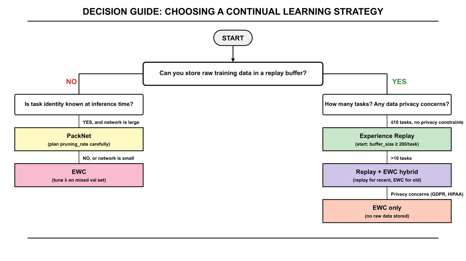
Raw data cannot be stored. This is the primary constraint in regulated industries. Healthcare models trained on patient records, fraud models trained on transaction data, and any system operating under GDPR or HIPAA typically cannot maintain a persistent buffer of historical training examples. Replay is structurally prohibited. Use EWC — it stores parameter statistics, not raw data.
Buffer is too small relative to task count. Reservoir sampling is uniform, but uniform over a growing pool. With 500 examples across 10 tasks, each task gets roughly 50 buffer slots on average. Whether 50 examples is enough depends on the task difficulty and the complexity of the distribution. For simple binary classification on well-separated data, it can be sufficient. For complex distributions with high intra-class variance, it is not. Scale buffer_size proportionally with n_tasks — budget at least 100–200 examples per task.
Class imbalance in the replay buffer. If Task 0 has 10,000 training examples and Task 1 has 500, reservoir sampling will still give them approximately equal buffer representation by Task 2. But during Task 1’s original training, Task 0’s examples dominate the buffer. This can cause the model to effectively train on a 50/50 mix of Task 0 and Task 1 data even when Task 1 data is scarce. Monitor the task distribution in the buffer after each task.
When PackNet breaks down
Task identity is unknown at inference. PackNet’s inference requires knowing which binary mask to apply before the forward pass. In task-incremental learning, the task ID is provided at inference time — this is the assumption the method is built on. In class-incremental learning (predict which of all K classes across all tasks) or domain-incremental learning (same output space, different input distributions), the task ID is not known. PackNet cannot function in these settings. Use EWC or replay.
More tasks than pruning_rate allows. The benchmark demonstrates this exactly. The rule: pruning_rate ≤ (T−1)/T. If you plan for T = 5 tasks and use pruning_rate = 0.5, you violate this rule immediately — after Task 2, later tasks are starved. Before deploying PackNet on a new task sequence, calculate the minimum free capacity for the final task: (1 − pruning_rate)^(T−1). If that number is below 0.15 (15% of the network), reduce pruning_rate or use a larger model.
Small networks. A 3-layer MLP with 50,000 parameters has less to partition than a ResNet-18 with 11 million. At 50% pruning on a small network, Task 3 may have fewer than 6,000 parameters available — insufficient for any non-trivial task. PackNet works best on large, over-parameterised networks where the free capacity after T tasks is still a large absolute number even if the percentage is small.
The Numbers in Context: What This Benchmark Is and Is Not
These results are from real benchmark runs on one architecture (multi-head MLP) and one dataset (Split-MNIST). The ordering — Replay > Baseline > EWC > PackNet — is specific to this setting. Across the continual learning literature, that ordering changes depending on:
- Architecture: single-head vs. multi-head, depth, width
- Task similarity: highly similar tasks favour EWC (more shared Fisher structure); dissimilar tasks favour replay
- Task count: EWC degrades gracefully but increasingly beyond Task 10; Replay scales well if buffer size scales with task count
- Dataset complexity: PackNet on ResNet-18 with 15% pruning on 10 tasks is a different story than PackNet on a 3-layer MLP with 50% pruning on 5 tasks
The benchmark in this article is designed to show the mechanics clearly, not to declare a universal winner. In your production system, the right method depends on your architecture, your data retention constraints, and how many tasks you plan to run over the model’s lifetime. The decision guide above is where to start. The benchmark code at benchmarks/benchmark.py is what to run on your actual data before committing to an approach.
Connecting to Production: Where This Fits in the Series
Article 03 built an ML retraining pipeline with drift-based triggers and an evaluation gate. Article 04 added a model registry with atomic promotion and rollback. This article adds the third piece: when the retraining pipeline fires and promotes a new model version, the continual learning methods here are what prevent that new model from forgetting the patterns the old model had learned.
In practice, the integration is straightforward. Your retraining pipeline from Article 03 trains the challenger model. Before that training begins, if you are using EWC, you run trainer.consolidate() on the current champion’s training data. If you are using replay, the buffer carries over between retraining runs. If you are using PackNet, the frozen masks are stored alongside the model artifact in the registry from Article 04.
The evaluation gate from Article 03 already checks both new-task performance and regression against the champion. In a continual learning system, you extend that gate: measure not just the new task’s metrics, but the accuracy on all prior task evaluation sets. If any prior task has dropped more than your configured threshold, the challenger fails the gate regardless of how well it performs on new data.
What Is Next
This article covers the foundational continual learning piece — the three primary strategies and when each applies. The next article in Cluster 2 goes deeper into the online learning variant of this problem: what happens when new data arrives as a continuous stream rather than discrete task batches, and how to update model weights incrementally without storing any data at all.
Article 06 — Online Learning in Python: How to Train Models on Streaming Data: covers the River library, SGD-based online learners, concept drift handling in streaming contexts, and evaluation strategies when there is no held-out set.
If your model is already deployed and degrading rather than starting fresh on continual learning, go directly to Article 09 — ML Model Monitoring to diagnose whether you are seeing concept drift, data drift, or catastrophic forgetting from a prior retraining cycle.
Complete Code: github.com/Emmimal/catastrophic-forgetting
References
[1] Mccloskey, M., & Cohen, N. J. (1989). Catastrophic interference in connectionist networks: The sequential learning problem. Psychology of Learning and Motivation, 24, 109–165. https://doi.org/10.1016/S0079-7421(08)60536-8
[2] Ratcliff, R. (1990). Connectionist models of recognition memory: Constraints imposed by learning and forgetting functions. Psychological Review, 97(2), 285–308. https://doi.org/10.1037/0033-295X.97.2.285
[3] Parisi, G. I., Kemker, R., Part, J. L., Kanan, C., & Wermter, S. (2019). Continual lifelong learning with neural networks: A review. Neural Networks, 113, 54–71. https://doi.org/10.1016/j.neunet.2019.01.012
[4] Kirkpatrick, J., Pascanu, R., Rabinowitz, N., Veness, J., Desjardins, G., Rusu, A. A., Milan, K., Quan, J., Ramalho, T., Grabska-Barwinska, A., Hassabis, D., Clopath, C., Kumaran, D., & Hadsell, R. (2017). Overcoming catastrophic forgetting in neural networks. Proceedings of the National Academy of Sciences, 114(13), 3521–3526. https://doi.org/10.1073/pnas.1611835114
[5] Robins, A. (1995). Catastrophic forgetting, rehearsal and pseudorehearsal. Connection Science, 7(2), 123–146. https://doi.org/10.1080/09540099550039318
[6] Mallya, A., & Lazebnik, S. (2018). PackNet: Adding multiple tasks to a single network by iterative pruning. Proceedings of the IEEE/CVF Conference on Computer Vision and Pattern Recognition Workshops (CVPRW). https://arxiv.org/abs/1711.05769
[7] Schwarz, J., Czarnecki, W., Luketina, J., Grabska-Barwinska, A., Teh, Y. W., Pascanu, R., & Hadsell, R. (2018). Progress & compress: A scalable framework for continual learning. Proceedings of the 35th International Conference on Machine Learning (ICML). https://arxiv.org/abs/1805.06370
[8] Vitter, J. S. (1985). Random sampling with a reservoir. ACM Transactions on Mathematical Software, 11(1), 37–57. https://doi.org/10.1145/3147.3165
[9] Lopez-Paz, D., & Ranzato, M. A. (2017). Gradient episodic memory for continual learning. Advances in Neural Information Processing Systems (NeurIPS), 30. https://proceedings.neurips.cc/paper/2017/hash/f87522788a2be2d171666752f97ddebb-Abstract.html
[10] Paszke, A., Gross, S., Massa, F., Lerer, A., Bradbury, J., Chanan, G., Killeen, T., Lin, Z., Gimelshein, N., Antiga, L., Desmaison, A., Kopf, A., Yang, E., DeVito, Z., Raison, M., Tejani, A., Chilamkurthy, S., Steiner, B., Fang, L., Bai, J., & Chintala, S. (2019). PyTorch: An imperative style, high-performance deep learning library. Advances in Neural Information Processing Systems (NeurIPS), 32. https://proceedings.neurips.cc/paper/2019/hash/bdbca288fee7f92f2bfa9f7012727740-Abstract.html
[11] LeCun, Y., Bottou, L., Bengio, Y., & Haffner, P. (1998). Gradient-based learning applied to document recognition. Proceedings of the IEEE, 86(11), 2278–2324. https://doi.org/10.1109/5.726791
Disclosure
Code authorship: All code in this article — the EWC trainer, Experience Replay buffer, PackNet implementation, MultiHeadMLP architecture, benchmark runner, CLMetrics, and test suite — is the original work of the author. The framework builds on PyTorch [10], an open-source deep learning library under the BSD license.
Benchmark authenticity: All benchmark numbers shown in this article are from real runs executed by the author on a CPU (Python 3.12, PyTorch 2.0+, Windows 10). The output shown in the benchmark table matches the logged output verbatim. No numbers were adjusted or estimated.
Dataset: The Split-MNIST benchmark uses the MNIST dataset [11], which is publicly available under a Creative Commons Attribution-Share Alike 3.0 license and is accessed via torchvision.datasets.MNIST.
No affiliate relationships: No tools, libraries, or services are mentioned for compensation. All recommendations reflect independent technical evaluation. All referenced tools are open-source under MIT or BSD licenses.
Series affiliation: This is Article 05 of the Production ML Engineering series published at EmiTechLogic. Articles 01–04 are linked where referenced.
Series: Production ML Engineering — Article 05 of 15 Previous: Model Versioning in Production Machine Learning (Article 04) Next: Online Learning in Python: How to Train Models on Streaming Data (Article 06)


")


Leave a Reply