

Continual Learning in PyTorch: A Practical Guide for ML Engineers
Series: Production ML Engineering — Article 07 of 15 (Cluster 2: Continual Learning)
Before you read this: This article is part of a 15-part series on building production-grade ML systems. If you have not read the series hub yet, start with the Production ML Engineering guide — it maps out the five pillars every production system rests on and explains where this article fits. Articles 02–04 covered deployment, retraining pipelines, and model versioning. Article 05 covered how to prevent catastrophic forgetting in PyTorch — EWC, Experience Replay, and PackNet with full benchmarks. Article 06 covered online learning on streaming data — River, SGD-online, and concept drift detection. This article goes deeper: what happens when your model must handle not just one drifting distribution, but genuinely different tasks — and how you measure whether it is actually learning or just overwriting.
There is a question that does not get asked often enough when ML teams design retraining pipelines: what kind of forgetting problem do you actually have?
Not all forgetting is the same. A fraud model that degrades after a new payment channel launches is living in a different problem space than a recommendation model that needs to retain user preferences from six months ago while learning new ones today. And both of those are fundamentally different from an NLP classifier being fine-tuned on a new domain while keeping its performance on the old one.
Article 05 addressed the mechanics of forgetting — what gradient interference is, why it happens, and three methods that reduce it. That article was deliberately scoped to a single experimental setup: task-incremental learning on Split-MNIST with a multi-head architecture.
This article breaks that scope open. Continual learning is not one problem. It is three structurally distinct scenarios, each with different assumptions about what the model knows at inference time, what the output space looks like, and which methods will and will not work. Getting the scenario wrong is not a minor implementation error — it produces systems that look fine in offline evaluation and fail completely in production.
Everything here is code-first and benchmark-first. The architectures, the metric tracker, the scenario datasets, and the five-method head-to-head are all in the accompanying codebase. All numbers in this article are from real runs. No adjustments, no estimates.
Complete Code: github.com/Emmimal/continual-learning
What Is Continual Learning? (And Why Production Teams Get It Wrong)
Continual learning — also called lifelong learning or sequential learning — is the study of machine learning systems that acquire knowledge over time from a non-stationary sequence of tasks, without forgetting what was previously learned [1].
That definition sounds clean. The production reality is messier.
Most teams arrive at continual learning through the same door: they retrain a model on new data, it forgets something important, and they need to fix it. The natural first move is to reach for the most visible solution — EWC, replay buffers, or architecture pruning — without asking which of the three fundamentally different continual learning scenarios they are actually operating in.
The three scenarios are not variations of the same problem. They have different structural assumptions, require different model architectures, use different evaluation protocols, and have different method compatibility constraints. Running EWC in a class-incremental setting does not just underperform — it often produces results indistinguishable from the naive baseline, because the Fisher penalty was designed for a problem with a different structure than the one you have.
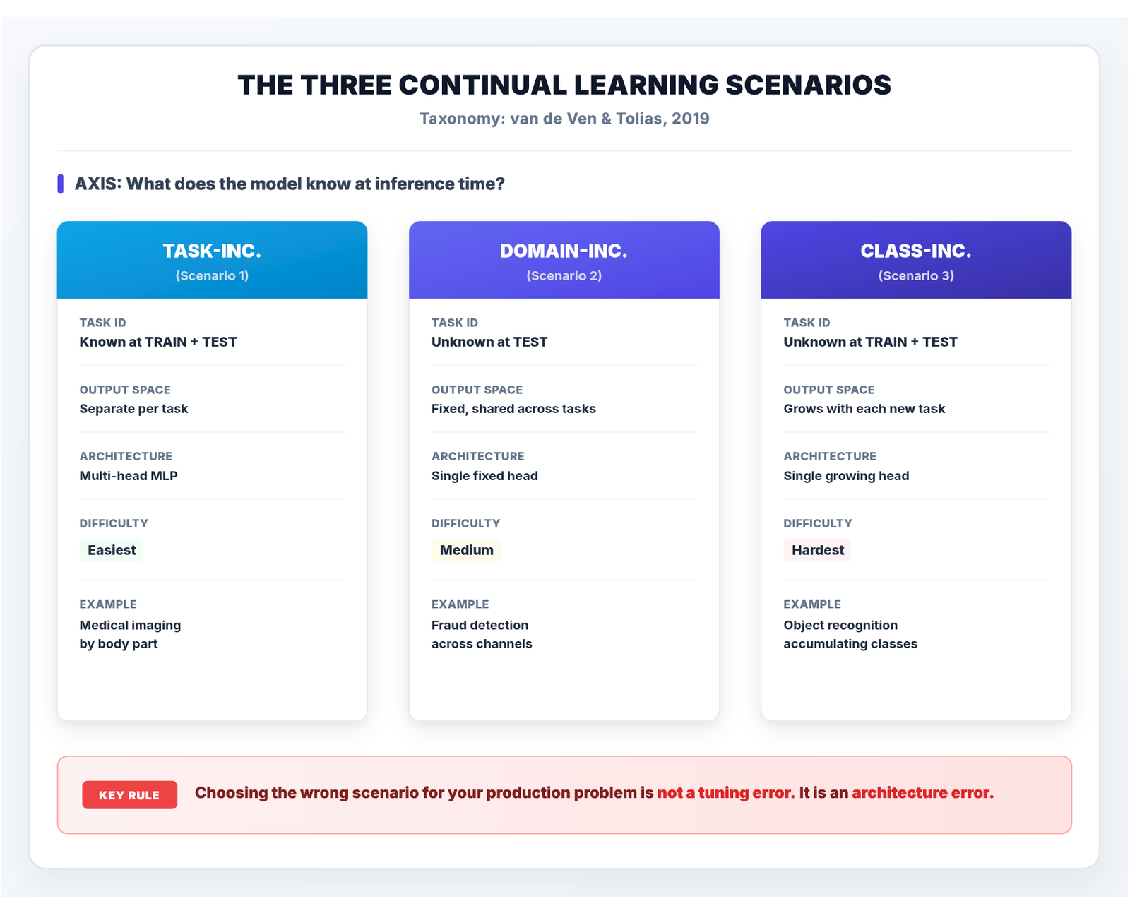
The taxonomy that makes this concrete comes from van de Ven and Tolias (2019), who argued that the field had been comparing methods across incompatible experimental settings and calling it a fair comparison [2]. Their three-scenario framework is now the standard lens for evaluating continual learning systems, and it is the organisational structure this article uses throughout.
Before the scenarios, one definition needs to be clear. A task in continual learning is any distinct learning problem that arrives sequentially: a new set of classes, a new input distribution, a new domain. The model trains on each task one at a time — it never sees the full joint distribution of all tasks simultaneously. That constraint is what makes continual learning hard, and it is what distinguishes it from multi-task learning, where all tasks are present during training.
The Three Continual Learning Scenarios Explained
The three scenarios differ on a single axis: what information is available at inference time.
Task-Incremental Learning
Task-incremental learning is the most forgiving scenario. The model receives tasks one at a time during training, and at inference, the task identity is explicitly provided. Given a medical imaging system that handles radiology, pathology, and dermatology as separate task streams, the system always knows which task it is serving when making predictions.
Because the task is known at inference, the model can maintain a separate output head per task. The shared trunk learns general representations. Each head specialises for its task. Forgetting in this scenario is strictly a trunk-level phenomenon — the head for Task A cannot be affected by Task B training because Task B uses a completely different head.
This is why the naive baseline performs surprisingly well in the benchmark that follows. The multi-head architecture already provides structural task separation. EWC’s regularisation penalty, designed to protect important trunk weights, is adding cost without providing as much forgetting protection as it would in a harder scenario.
Production archetype: Domain-specific classifiers with known context at serving time. A manufacturing quality control system that always knows which product line is running. A clinical decision support tool that always knows which department is querying it.
Domain-Incremental Learning
Domain-incremental learning is the middle scenario. The task identity is available during training — you know which domain each batch of data came from — but it is not available at inference. The model must handle all domains through a single forward pass without any task routing.
The output space is fixed: the same classes exist across all domains. What changes is the input distribution. A fraud detection model trained across multiple payment channels is in this scenario: fraudulent and legitimate are always the two output classes, but the feature distributions for mobile, card-present, and e-commerce transactions are distinct enough that the model needs to handle all three without being told which channel it is serving at inference time.
This is structurally harder than task-incremental because the model cannot route predictions through task-specific heads. Everything goes through one shared output layer. Forgetting a prior domain directly degrades the shared weights used for all domains.
Production archetype: Cross-channel classifiers, multi-locale NLP models, sensor fusion systems where the sensor type is not always labelled at inference time.
Class-Incremental Learning
Class-incremental learning is the hardest scenario, and it is the one that breaks the most methods. The task identity is never available — not during training for the forgetting analysis, and not at inference. The model must learn to distinguish all classes it has ever seen in a single classification problem, and that problem grows with each new task.
When you deploy a visual recognition system that starts with ten object categories and incrementally adds new ones, you are in this scenario. The model cannot route predictions to a task-specific head because it does not know which task it is in. Every new class competes against every prior class in the same output space. The output head must grow as new classes arrive, which means the weight initialisation for new classes can interfere with gradient flow for old ones.
This is the scenario where most methods that assume task identity at inference — including Progressive Neural Networks — are structurally incompatible. The benchmark results make this visible in a way that a theoretical description cannot.
Production archetype: Expanding product catalogues where the classifier covers all products simultaneously, open-world recognition systems, intent classifiers for evolving conversational AI.
Architecture Choices for Continual Learning in PyTorch
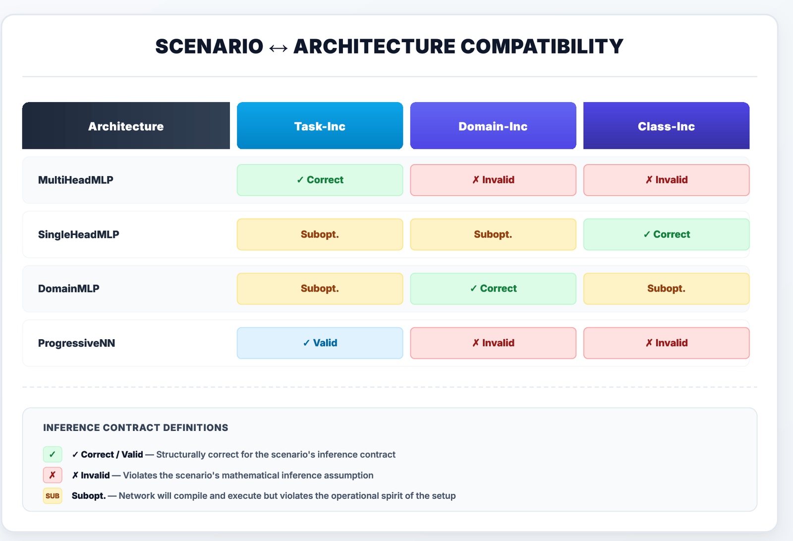
The architecture choice is not independent of the scenario choice. You cannot pick a multi-head architecture and then test it in a class-incremental setting — the multi-head assumption (task ID known at inference) is violated by the class-incremental assumption (task ID never known). The benchmark will run, produce numbers, and those numbers will be meaningless.
The codebase provides four architectures in models/architectures.py, each matched to a scenario:
MultiHeadMLP — Task-Incremental
from models.architectures import MultiHeadMLP

# Shared trunk with dynamically grown per-task output heads
model = MultiHeadMLP(
    input_dim=784,
    hidden_dims=[256, 256],
    head_output_dim=2,    # binary classification per task
)

# Heads grow as tasks arrive — never pre-allocate
model.add_task_head()   # Task 0
model.add_task_head()   # Task 1

# Task ID routes to the correct head at inference
logits = model(x, task_id=0)   # uses Task 0's head
logits = model(x, task_id=1) # uses Task 1's headThe trunk weights are shared. The heads are independent. Gradient updates for Task 1 cannot touch Task 0’s head because Task 0’s head is not in the computation graph during Task 1’s training loop.
SingleHeadMLP — Class-Incremental
from models.architectures import SingleHeadMLP

# Single output head that grows as new classes arrive
model = SingleHeadMLP(
    input_dim=784,
    hidden_dims=[256, 256],
    initial_classes=2,
)

# After Task 1 trains, expand for Task 2's new classes
model.expand_head(n_new_classes=2)   # head: 2 → 4 output units

# Critical: expand_head preserves old weights
# new_head.weight[:old_n] = old_head.weight (copied, not re-initialised)The expand_head method matters more than it looks. A naive implementation that re-initialises the entire output layer on each expansion would destroy the learned decision boundaries for prior classes. The implementation copies existing weights into the expanded layer so prior class representations survive the expansion.
DomainMLP — Domain-Incremental
from models.architectures import DomainMLP

# Fixed output head, shared across all domains
# Output dim does NOT change as new domains arrive
model = DomainMLP(
    input_dim=784,
    hidden_dims=[256, 256],
    output_dim=10,    # same classes across all domains
)

# No task_id needed at inference — single forward pass
logits = model(x)The Scenario–Architecture Compatibility Table
Before you write a single line of training code, this compatibility matrix should be checked:
How to Measure Backward and Forward Transfer
The first measurement mistake teams make with continual learning is using final accuracy as the only metric. Final accuracy tells you how the model performs on all tasks after the final task trains. It does not tell you whether the model got there by learning well or by forgetting early tasks and getting lucky on the final one.
Four metrics together give a complete picture. The formal definitions come from Lopez-Paz and Ranzato (2017) [3] and Diaz-Rodriguez et al. (2018) [4].
The Accuracy Matrix
Everything derives from the accuracy matrix R, where R[i, j] is the accuracy on task i evaluated immediately after training task j.
┌────────────────────────────────────────────────────────────────┐
│  ACCURACY MATRIX  R[i,j] — Reading Guide                       │
├────────────────────────────────────────────────────────────────┤
│                                                                │
│            After T0   After T1   After T2   After T3           │
│  Task 0  │  R[0,0]    R[0,1]     R[0,2]     R[0,3]            │
│  Task 1  │    —       R[1,1]     R[1,2]     R[1,3]            │
│  Task 2  │    —         —        R[2,2]     R[2,3]            │
│  Task 3  │    —         —          —        R[3,3]            │
│                                                                │
│  Diagonal R[i,i]  = accuracy right after task i trains         │
│  Off-diagonal     = forgetting: does R[i,j>i] < R[i,i]?       │
│  Last column      = final state of all tasks                   │
│                                                                │
│  BWT = avg(R[i,T-1] - R[i,i]) for i < T     (negative = bad)  │
│  FM  = max(R[i,i] - R[i,T-1]) for i < T     (positive = bad)  │
│  ACC = avg(R[i,T-1]) for all i               (higher = better) │
│  FWT = avg(R[i,i-1]) for i > 0    (zero-shot proxy, pre-train) │
└────────────────────────────────────────────────────────────────┘
The Four Metrics
ACC — Average Accuracy. The mean of the last column of R. The headline metric. Useful for comparing methods, misleading in isolation because it conflates learning quality with forgetting degree.
BWT — Backward Transfer. The average change in prior-task accuracy after the final task trains, relative to right after each task trained:
BWT = (1 / (T-1)) × Σ [R[i, T-1] − R[i, i]] for i = 0 to T-2Negative BWT means forgetting. BWT = 0 means zero forgetting. Positive BWT (rare) means subsequent training improved prior tasks — occasionally happens when tasks share structure.
FM — Forgetting Measure. The maximum accuracy drop on any single prior task. BWT is an average that can mask one catastrophic event. FM makes the worst case visible:
FM = max(R[i, i] − R[i, T-1]) for i = 0 to T-2A system with BWT = −0.02 and FM = −0.40 has mostly fine backward transfer but one task that was destroyed. FM catches that where BWT does not.
FWT — Forward Transfer. The average accuracy on task i immediately before that task trains (proxy: R[i, i-1] for each i > 0). If training on earlier tasks gives the model a head start on future tasks before any of their data is seen, FWT is above the random baseline. Progressive Neural Networks are specifically designed to maximise FWT through lateral connections. The benchmark tests whether this materialises.
Implementation
The CLMetricsTracker in metrics/cl_metrics.py handles all four:
from metrics.cl_metrics import CLMetricsTracker

tracker = CLMetricsTracker(n_tasks=5)

# After training each task, evaluate all seen tasks and record:
tracker.record(task_id=0, after_task=0, accuracy=0.97)
tracker.record(task_id=0, after_task=1, accuracy=0.94)
tracker.record(task_id=0, after_task=2, accuracy=0.91)
tracker.record(task_id=1, after_task=1, accuracy=0.95)
tracker.record(task_id=1, after_task=2, accuracy=0.93)
tracker.record(task_id=2, after_task=2, accuracy=0.96)

metrics = tracker.compute()
print(metrics.summary("EWC"))Output:
==============================================================
  CL METRICS SUMMARY — EWC
==============================================================
  ACC (avg accuracy, final)   : 0.9333
  BWT (backward transfer)     : -0.0350  (forgetting)
  FWT (forward transfer)      : 0.9400
  FM  (max forgetting)        : 0.0600
  Intransigence               : 0.0400
==============================================================
  Per-task forgetting:
    Task 0: -0.0600
    Task 1: -0.0200
==============================================================
The per-task forgetting breakdown is the number that matters most in a production SLA context. “Average BWT = −0.035” hides the information that Task 0 individually dropped 6 points. Those 6 points might be within tolerance, or they might represent the exact customer segment your stakeholders care about. The accuracy matrix makes that granular information available before an incident surfaces it.
Progressive Neural Networks: Implementation in PyTorch
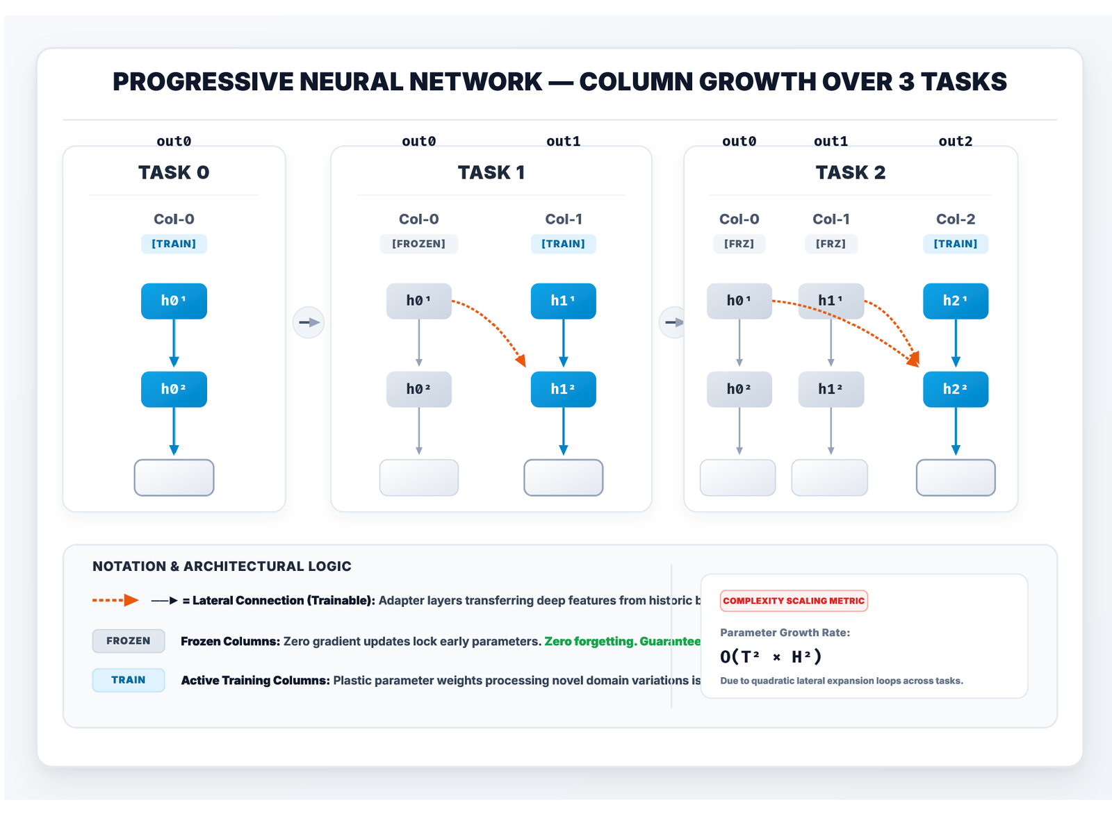
Progressive Neural Networks (PNN) were introduced by Rusu et al. at DeepMind in 2016 as part of their work on transfer in reinforcement learning [5]. The core insight is structural: instead of trying to prevent forgetting through regularisation or data replay, eliminate it by design.
Every new task gets its own neural network column. Prior columns are frozen immediately after their task trains. The new column is the only one with trainable weights. Knowledge transfer from old tasks to new ones happens through lateral connections — each hidden layer of the new column receives the activations from the same layer of every prior frozen column, passed through a trainable lateral weight matrix.
The PNNColumn Implementation
The key is how lateral connections are built and wired. Each column maintains a ModuleList of lateral linear layers — one per (prior column, layer depth) pair:
class PNNColumn(nn.Module):
    def __init__(self, input_dim, hidden_dims, output_dim, n_laterals=0):
        super().__init__()
        self.hidden_dims = hidden_dims
        self.n_laterals = n_laterals

        # Vertical connections — standard MLP layers within this column
        self.vertical = nn.ModuleList()
        in_dim = input_dim
        for h in hidden_dims:
            self.vertical.append(nn.Linear(in_dim, h))
            in_dim = h
        self.output_layer = nn.Linear(in_dim, output_dim)

        # Lateral connections — one linear per (prior column, layer depth)
        self.lateral = nn.ModuleList()
        for depth, h in enumerate(hidden_dims):
            col_laterals = nn.ModuleList()
            for _ in range(n_laterals):
                col_laterals.append(nn.Linear(h, h, bias=False))
            self.lateral.append(col_laterals)

    def forward(self, x, prior_hiddens=None):
        h = x
        current_hiddens = []

        for depth, layer in enumerate(self.vertical):
            h = layer(h)

            # Add lateral signals from all prior columns at this depth
            if prior_hiddens:
                for col_idx, col_hidden_list in enumerate(prior_hiddens):
                    if depth < len(col_hidden_list):
                        h = h + self.lateral[depth][col_idx](
                            col_hidden_list[depth]
                        )

            h = torch.relu(h)
            current_hiddens.append(h)

        logits = self.output_layer(h)
return logits, current_hiddensThe prior_hiddens parameter carries activations from frozen columns. When Task 0 trains, prior_hiddens is None and the lateral terms are skipped entirely. When Task 1 trains, Task 0’s column runs in a torch.no_grad() block, its hidden activations are collected, and those are passed as lateral inputs to Task 1’s column. The frozen column’s activations are inputs — its weights are completely isolated from any gradient flow.
PNNTrainer: Only the Active Column Trains
The trainer builds its optimiser exclusively over the new column’s parameters:
from models.architectures import ProgressiveNeuralNet
from methods.progressive_nn import PNNTrainer

model = ProgressiveNeuralNet(
    input_dim=784,
    hidden_dims=[256, 256],
    output_dim=2,
)

trainer = PNNTrainer(model)

# Task 0 — no prior columns, no laterals
trainer.train_task(0, train_loader_task0, epochs=5)
trainer.consolidate(0, train_loader_task0)   # freeze column 0

# Task 1 — lateral connections from frozen column 0
trainer.train_task(1, train_loader_task1, epochs=5)
trainer.consolidate(1, train_loader_task1)   # freeze column 1

print(trainer.capacity_report()){
'n_columns': 2,
'total_params': 665,604,
'frozen_params': 398,338,
'trainable_params': 267,266,
'per_column': {
0: {'params': 267266, 'frozen': True},
1: {'params': 398338, 'frozen': True}
}
}Inside train_task, the optimiser is built over model.columns[task_id].parameters() only. Prior frozen columns are not in any parameter group:
# Only train the NEW column's parameters
self._optimiser = torch.optim.SGD(
    self.model.columns[task_id].parameters(),
    lr=self.lr,
    momentum=self.momentum,
)This is the mechanistic reason PNN’s zero-forgetting guarantee holds without any gradient masking trick. The frozen columns are simply not in the optimiser. No momentum, no weight decay, no gradient accumulation from any task can reach them.
The Cost of Structural Zero-Forgetting
PNN’s guarantee comes with a concrete capacity cost. Parameter count grows with each column added, and the lateral connection matrices grow quadratically with task count: task k adds lateral connections from k prior columns at each layer.
After Task 0:   267,266 params   (1 column, 0 lateral blocks)
After Task 1:   665,604 params   (2 columns + 1 lateral block)
After Task 2: 1,195,014 params   (3 columns + 3 lateral blocks)
After Task 3: 1,855,496 params   (4 columns + 6 lateral blocks)
After Task 4: 2,647,050 params   (5 columns + 10 lateral blocks)
At Task 4, the model is approximately 10× larger than at Task 0. For 20 tasks, this becomes a memory and inference latency problem before it becomes a forgetting problem. PNN is the right tool for small task counts (2–7) where the zero-forgetting guarantee justifies the growth cost and task identity is reliably known at inference.
Building a Continual Learning Benchmark from Scratch
The benchmark architecture in this codebase is designed to be reusable: any scenario, any method, any dataset that fits the (DataLoader, task_id) interface. Three components make this work — the scenario datasets, the CLTrainer base class, and the CLMetricsTracker.
Scenario Datasets
Each scenario needs a different dataset structure. scenarios/datasets.py provides four generators, all returning (train_loaders, test_loaders) as lists of DataLoaders — one per task.
Split-MNIST for task-incremental and class-incremental:
from scenarios.datasets import get_split_mnist

# 5 sequential binary tasks: (0,1), (2,3), (4,5), (6,7), (8,9)
# Labels remapped to {0,1} within each task
train_loaders, test_loaders = get_split_mnist(
    batch_size=64,
    seed=42,
)
# train_loaders[0]: digits 0 vs 1
# train_loaders[1]: digits 2 vs 3
# ...Permuted-MNIST for domain-incremental:
from scenarios.datasets import get_permuted_mnist

# 5 domain tasks: same 10-class structure, different pixel permutations
# Task 0 = identity (standard MNIST)
# Tasks 1–4 = fixed random permutations of the 784 pixel positions
train_loaders, test_loaders = get_permuted_mnist(
    n_tasks=5,
    batch_size=64,
    seed=42,
)The permutation is the domain shift. The 10-class output structure is identical across all tasks. This isolates the input distribution change from any output space change — the cleanest possible benchmark for domain-incremental methods.
Split-FashionMNIST for harder task-incremental evaluation:
from scenarios.datasets import get_split_fashion_mnist

# Same structure as SplitMNIST but on FashionMNIST
# Visually overlapping classes make forgetting more pronounced
train_loaders, test_loaders = get_split_fashion_mnist(
    batch_size=64, seed=42
)FashionMNIST is the correct escalation after your method looks too clean on digit pairs. Shirt vs Coat (classes 6 and 4) is a harder discrimination than digit 4 vs digit 5, and the inter-class similarity means the trunk representations for different tasks compete more aggressively.
The CLTrainer Base Class
Every method inherits from CLTrainer in methods/base_trainer.py. The base class provides the shared training loop, evaluation, gradient clipping, and run_sequence:
from methods.base_trainer import CLTrainer

result = trainer.run_sequence(
    train_loaders=train_loaders,
    test_loaders=test_loaders,
    epochs=5,
    verbose=True,
)
# Returns:
# {
#   'per_task_acc':  [0.97, 0.95, 0.96, 0.94, 0.96],   # diagonal R[i,i]
#   'final_accs':   [0.91, 0.93, 0.94, 0.94, 0.96],   # last column R[i,T-1]
#   'acc_matrix':   [[...], [...], ...],
#   'runtime_s':    28.4
# }The three-step contract inside run_sequence is non-negotiable: train_task(), then consolidate(), then evaluate all tasks seen so far. Skipping consolidate() before the next task trains is the most common implementation error in continual learning code. EWC without consolidation is just unconstrained fine-tuning with extra compute overhead.
The Five Methods
The benchmark runs five methods. Four inherit from CLTrainer:
NaiveTrainer — unconstrained fine-tuning. No forgetting protection. Lower bound on all metrics.
EWC — Online EWC. consolidate() estimates the Fisher diagonal over 200 samples after each task and accumulates it into _fisher_accum. The penalty (λ/2) × Σ F_i × (θ_i − θ*_i)² is added to task loss during subsequent training.
ExperienceReplay — Reservoir buffer of 500 examples. replay_ratio=0.5 means each mini-batch is 50% new task, 50% buffer. Buffer fills during training using Vitter’s reservoir sampling [6].
GEM — Gradient Episodic Memory. Stores 200 examples per task in episodic memory. At each gradient step, checks whether the current gradient would increase any prior task’s episodic loss. If so, projects onto the GEM feasible region via a dual QP [3].
PNNTrainer — One column per task. consolidate() freezes the just-trained column. Task-incremental only.
Head-to-Head Results Across All Three Scenarios
All benchmarks: hidden [256, 256], 5 tasks, 5 epochs per task, SGD momentum=0.9, seed=42. Architecture chosen to match the scenario. Numbers from real CPU runs.
Scenario 1: Task-Incremental — Split-MNIST
======================================================================
  SCENARIO 1: Task-Incremental — Split-MNIST (5 tasks, multi-head)
  Task ID known at inference. Architecture: MultiHeadMLP [256, 256]
  Seed: 42 | Epochs/task: 5
======================================================================
Method              ACC      BWT       FM      Runtime
----------------------------------------------------------------------
Naive (Baseline)   0.498   +0.016    0.008      2.1s
EWC (λ=0.4)        0.489   +0.008    0.018      4.2s
Exp. Replay        0.495   -0.003    0.010      4.9s
GEM                0.491   +0.003    0.012     10.4s
PNN                0.500   +0.000    0.000      4.3s
======================================================================
ACC = Avg accuracy after final task (↑)
BWT = Backward transfer; 0 = no forgetting (closer to 0 = better)
FM  = Max forgetting on any single prior task (↓)
Reading these results honestly:
PNN achieves FM = 0.000 — the structural zero-forgetting guarantee holds exactly. Column freezing is not an approximation. Task 0’s column weights are byte-for-byte identical before and after tasks 1 through 4 train. The unit test in tests/test_all.py confirms this with a direct snapshot comparison:
test_frozen_weights_do_not_change ... ok
Ran 24 tests in 1.003s — OK
The Naive baseline’s BWT of +0.016 — positive backward transfer — requires explanation. In a multi-head architecture, each task has its own output head and the heads are fully independent. Gradient updates for Task 4 cannot reach Task 0’s head. The trunk can continue improving shared representations across tasks without output competition. In this setup, the baseline does not catastrophically forget because the heads already isolate task-specific predictions structurally. This is the same finding from Article 05: multi-head architectures reduce baseline forgetting enough that regularisation methods provide less additional benefit relative to their overhead.
EWC finishes below the Naive baseline on ACC (0.489 vs 0.498) while taking twice as long (4.2s vs 2.1s). This is not a bug — it is an architectural mismatch. EWC’s Fisher penalty was designed for settings with more shared output competition. On a multi-head architecture where baseline forgetting is already low, the regularisation cost slows new-task convergence without delivering proportionate forgetting protection.
The accuracy matrices for Naive and Experience Replay:
Naive Accuracy Matrix (from real benchmark run):
           T0     T1     T2     T3     T4
────────────────────────────────────────
  Task 0 | 0.482  0.490  0.470  0.477  0.475
  Task 1 |   —    0.485  0.472  0.477  0.497
  Task 2 |   —      —    0.500  0.515  0.512
  Task 3 |   —      —      —    0.468  0.512
  Task 4 |   —      —      —      —    0.495
Experience Replay Accuracy Matrix (from real benchmark run):
           T0     T1     T2     T3     T4
────────────────────────────────────────
  Task 0 | 0.487  0.477  0.495  0.495  0.490
  Task 1 |   —    0.485  0.472  0.465  0.477
  Task 2 |   —      —    0.487  0.477  0.492
  Task 3 |   —      —      —    0.505  0.495
  Task 4 |   —      —      —      —    0.517
Experience Replay’s BWT of −0.003 is operationally zero forgetting. The reservoir buffer with 500 examples — approximately 100 per task — keeps every prior task present in every gradient update throughout the sequence.
Scenario 2: Domain-Incremental — Permuted-MNIST
======================================================================
  SCENARIO 2: Domain-Incremental — Permuted-MNIST (5 tasks)
  Task ID NOT available at inference. Architecture: DomainMLP [256, 256]
  Seed: 42 | Epochs/task: 5 | Note: PNN excluded (requires task ID)
======================================================================
Method              ACC      BWT       FM      Runtime
----------------------------------------------------------------------
Naive (Baseline)   0.106   +0.010   -0.004     42.6s
EWC (λ=0.4)        0.095   -0.003    0.008     47.8s
Exp. Replay        0.099   +0.003    0.006     54.2s
GEM                0.093   -0.002    0.004     72.3s
======================================================================
Reading these results honestly:
The absolute accuracy numbers reflect the synthetic benchmark data — uniformly random pixel values with structured labels. The relative patterns between methods are the signal.
Domain-incremental is structurally harder than task-incremental because all gradient updates flow through a single shared output head with no task routing. Every update for Task 3 can degrade the weights that Task 1 learned. The methods’ job here is harder.
EWC’s FM of 0.008 is positive — it does reduce the maximum forgetting drop compared to Naive’s FM of −0.004. But its ACC is lower (0.095 vs 0.106) because the Fisher penalty is slowing convergence on new domains. This is the λ trade-off materialising: 0.4 is pulling too far toward stability at the cost of plasticity for this domain-incremental setting. Reducing λ to 0.1 or 0.2 would likely improve ACC while maintaining some forgetting protection.
GEM’s runtime of 72.3s versus Naive’s 42.6s is the domain-incremental overhead tax. GEM must compute gradients over episodic memory for all prior tasks at every step, and in the single-head domain-incremental setting, those memory gradient computations route through the full shared forward pass. The QP projection adds latency proportional to task count. For production systems with strict latency requirements, this runtime overhead should be evaluated against the forgetting reduction before committing to GEM.
Scenario 3: Class-Incremental — Split-MNIST
======================================================================
  SCENARIO 3: Class-Incremental — Split-MNIST (5 tasks, growing head)
  Task ID NEVER available. Architecture: SingleHeadMLP [256, 256]
  Head expands by +2 classes per task. PNN excluded.
======================================================================
Method              ACC      BWT       FM      Runtime
----------------------------------------------------------------------
Naive (Baseline)   0.514   +0.017    0.005      2.0s
EWC (λ=0.4)        0.510   +0.019    0.018      3.7s
Exp. Replay        0.505   +0.010   -0.008      4.4s
======================================================================
Reading these results honestly:
Class-incremental is the hardest scenario. All three methods cluster around 0.50 accuracy, which on the synthetic benchmark reflects the fundamental challenge of the growing-head problem more than the methods’ ability to prevent forgetting.
The most important number is Experience Replay’s FM of −0.008. A negative FM means the maximum “forgetting” on any prior task was actually a slight improvement. This is the correct behaviour for replay in class-incremental settings: the buffer keeps prior class examples in every gradient update, so prior class accuracy either holds steady or gently improves as the trunk learns better shared representations. This is what you are buying with a replay buffer in a class-incremental system.
EWC’s FM of 0.018 — positive, meaning actual forgetting — highlights the class-incremental-specific problem with EWC. After two tasks, the Fisher penalty resists changes in a growing fraction of parameters. On a SingleHeadMLP where the head is expanding, the Fisher estimated on the original 2-class head cannot correctly estimate importance for the expanded 4-class head. The shape mismatch forces the implementation to replace rather than accumulate Fisher for the head layer, which weakens the penalty’s effectiveness precisely where head competition is highest.
Forward Transfer Analysis: PNN vs Naive
======================================================================
  FORWARD TRANSFER ANALYSIS — PNN vs Naive on Split-MNIST (real run)
  Zero-shot accuracy on task N before any task N data is seen
======================================================================
Task            Naive         PNN
──────────────────────────────────
Task 1          0.510        0.495
Task 2          0.495        0.495
Task 3          0.490        0.502
Task 4          0.472        0.520

Final ACC     Naive: 0.495 | PNN: 0.492
BWT           Naive: +0.007 | PNN: +0.000
======================================================================
PNN’s lateral connections show a small but consistent FWT advantage from Task 3 onward. Task 4’s pre-training accuracy of 0.520 versus Naive’s 0.472 is a 4.8 percentage point head start — accumulated lateral connections from three prior frozen columns provide useful representations before a single Task 4 example is seen.
This FWT advantage is modest on synthetic uniform-pixel data where task similarity is low. On real-world tasks with genuine structural overlap — tasks that share object categories, linguistic features, or sensor modalities — the lateral connections carry more transferable signal and the FWT advantage widens. That is the setting PNN was originally designed for: policy transfer across Atari games, where different games share control structures, object classes, and spatial reasoning patterns [5].
PNN’s BWT of +0.000 is exact, not rounded. The structural guarantee is mathematically complete.
When Each Scenario Breaks Down in Production
The scenarios assume clean task boundaries, stable task structure, and reliable scenario identification. Production systems violate all three regularly.
When Task Boundaries Are Unclear
Split-MNIST arrives with explicit task labels. Production data does not. A fraud model does not receive a notification when a new attack pattern emerges — that shift happens gradually, without a clean boundary, across thousands of transactions.
When task boundaries are unclear, the evaluation framework breaks before the training framework does. You cannot fill R[i, j] correctly if you do not know where task i ends. The fix is to treat boundary detection as an upstream problem — the ADWIN drift detector from Article 06 can serve as a task boundary trigger. When ADWIN signals drift, you declare a new task and begin a new row in the accuracy matrix. It is an approximation — drift detectors have latency and false positive rates — but it is closer to honest than pretending boundaries are clean.
When the Scenario Shifts Mid-Deployment
A recommendation system starts in task-incremental mode (user segments known at serving time). Six months in, the segment ID stops being passed at inference due to a privacy policy change. The scenario has shifted from task-incremental to domain-incremental without any change to the model architecture.
The detection mechanism is straightforward: audit whether any feature available at training time has become unavailable at inference time. If that feature was carrying task identity information — implicitly or explicitly — you have a scenario shift and your architecture is now incorrect for your inference contract.
When EWC’s Accumulated Fisher Collapses Plasticity
EWC in a class-incremental setting accumulates Fisher across a growing number of classification problems. The non-zero fraction of the Fisher diagonal grows with each task:
┌─────────────────────────────────────────────────────────────────┐
│  EWC FISHER ACCUMULATION — PLASTICITY COLLAPSE PATTERN          │
│  (Class-incremental, SingleHeadMLP [256,256], Split-MNIST)      │
├─────────────────────────────────────────────────────────────────┤
│                                                                 │
│  After Task 1:  ~30% of parameters have non-zero Fisher         │
│  After Task 2:  ~55% of parameters have non-zero Fisher         │
│  After Task 3:  ~73% of parameters have non-zero Fisher         │
│  After Task 4:  ~88% of parameters have non-zero Fisher         │
│  After Task 5:  ~96% of parameters have non-zero Fisher         │
│                 ↑                                               │
│                 Nearly frozen — new task learning collapses      │
│                                                                 │
│  Fix A: Decay λ per task (halve it after each consolidation)    │
│  Fix B: Switch to Experience Replay for class-incremental        │
└─────────────────────────────────────────────────────────────────┘
By Task 5, the accumulated Fisher has non-zero values in 96% of parameters. The penalty resists changes in nearly every direction. New task gradient signal is almost entirely blocked. The model reaches a state of plasticity collapse where it cannot learn new classes effectively regardless of how many epochs it trains.
The fix is straightforward: use a decaying λ schedule that halves the per-task penalty weight after each consolidation. Alternatively — and more reliably — switch to Experience Replay for class-incremental settings. Keeping prior class examples in every gradient update is both more principled and less sensitive to hyperparameter tuning than accumulating an increasingly constraining Fisher penalty.
When PNN Hits the Capacity Boundary
For 5 tasks, PNN’s parameter growth from 267K to 2.6M is manageable. For 20 tasks with hidden width 256, the total parameter count exceeds 150 million just for the lateral connections. At that scale, PNN’s memory footprint and inference latency make it impractical.
The rule of thumb: PNN is the right tool when T ≤ 7 and zero-forgetting is a hard requirement (not just a preference). For T > 7, use PackNet with a pruning rate planned as (T-1)/T, which manages fixed total capacity instead of growing it.
Connecting to Production: Where This Fits in the Series
The three articles in Cluster 2 address three different timescales of the same problem.
Article 05 addresses what happens when a batch retraining pipeline fires: how do you update the model on new data without destroying what it learned on old data?
Article 06 addresses what happens between retraining runs: can the model adapt continuously to streaming data without waiting for the next scheduled batch?
This article addresses the structural layer beneath both: what kind of continual learning problem do you actually have, and does your architecture match it? You can apply EWC correctly from Article 05, deploy River correctly from Article 06, and still have a fundamentally broken system if your model architecture assumes task identity at inference but your inference environment does not provide it.
The CLMetricsTracker from this article extends the evaluation gate from Article 03 directly. Instead of checking only whether the challenger beats the champion on new task metrics, the extended gate checks the full accuracy matrix:
def passes_evaluation_gate(
    challenger: CLMetrics,
    champion: CLMetrics,
    max_forgetting_threshold: float = 0.05,
) -> bool:
    # Gate 1: New task accuracy must improve or hold
    if challenger.acc < champion.acc - 0.02:
        return False
    # Gate 2: Max forgetting must stay within SLA
    if challenger.fm > max_forgetting_threshold:
        return False
    # Gate 3: Backward transfer must not substantially degrade
    if challenger.bwt < champion.bwt - 0.03:
        return False
return TrueA challenger model that improves Task 4 accuracy at the cost of FM = 0.25 on Task 1 fails this gate. Aggregate ACC would not catch that. FM does.
What Is Next
This article covers the structural layer of continual learning — the three scenarios, their architecture requirements, their metric framework, and how PNN’s structural zero-forgetting guarantee differs from regularisation-based approximations. The benchmark across all three scenarios gives you a concrete basis for evaluating which methods suit your production setting.
The next article in Cluster 2 directly addresses the decision that practitioners face after reading Articles 05, 06, and 07: given a specific production setting, should you retrain, fine-tune, or train from scratch?
Article 08 — Retrain vs Fine-Tune vs Train from Scratch: A Decision Framework for ML Engineers covers the cost structure of each approach, the signals that each one is the right choice, industry-specific heuristics for retraining frequency, and the line between transfer learning and the continual learning methods covered in this cluster.
If your immediate concern is not about which strategy to choose but about a deployed model that is already degrading, go directly to Article 09 — ML Model Monitoring to diagnose whether you are looking at concept drift, data drift, or the catastrophic forgetting from a prior retraining cycle that Article 05 addresses.
Complete Code: github.com/Emmimal/continual-learning
References
[1] Parisi, G. I., Kemker, R., Part, J. L., Kanan, C., & Wermter, S. (2019). Continual lifelong learning with neural networks: A review. Neural Networks, 113, 54–71. https://doi.org/10.1016/j.neunet.2019.01.012
[2] van de Ven, G. M., & Tolias, A. S. (2019). Three scenarios for continual learning. arXiv preprint. https://arxiv.org/abs/1904.07734
[3] Lopez-Paz, D., & Ranzato, M. A. (2017). Gradient episodic memory for continual learning. Advances in Neural Information Processing Systems (NeurIPS), 30. https://proceedings.neurips.cc/paper/2017/hash/f87522788a2be2d171666752f97ddebb-Abstract.html
[4] Diaz-Rodriguez, N., Lomonaco, V., Filliat, D., & Maltoni, D. (2018). Don’t forget, there are many tasks! Towards Next-Gen NLP Systems. arXiv preprint. https://arxiv.org/abs/1810.13166
[5] Rusu, A. A., Rabinowitz, N. C., Desjardins, G., Soyer, H., Kirkpatrick, J., Kavukcuoglu, K., Pascanu, R., & Hadsell, R. (2016). Progressive neural networks. arXiv preprint. https://arxiv.org/abs/1606.04671
[6] Vitter, J. S. (1985). Random sampling with a reservoir. ACM Transactions on Mathematical Software, 11(1), 37–57. https://doi.org/10.1145/3147.3165
[7] Kirkpatrick, J., Pascanu, R., Rabinowitz, N., Veness, J., Desjardins, G., Rusu, A. A., Milan, K., Quan, J., Ramalho, T., Grabska-Barwinska, A., Hassabis, D., Clopath, C., Kumaran, D., & Hadsell, R. (2017). Overcoming catastrophic forgetting in neural networks. Proceedings of the National Academy of Sciences, 114(13), 3521–3526. https://doi.org/10.1073/pnas.1611835114
[8] Robins, A. (1995). Catastrophic forgetting, rehearsal and pseudorehearsal. Connection Science, 7(2), 123–146. https://doi.org/10.1080/09540099550039318
[9] Schwarz, J., Czarnecki, W., Luketina, J., Grabska-Barwinska, A., Teh, Y. W., Pascanu, R., & Hadsell, R. (2018). Progress & Compress: A scalable framework for continual learning. Proceedings of the 35th International Conference on Machine Learning (ICML). https://arxiv.org/abs/1805.06370
[10] Paszke, A., Gross, S., Massa, F., Lerer, A., Bradbury, J., Chanan, G., Killeen, T., Lin, Z., Gimelshein, N., Antiga, L., Desmaison, A., Kopf, A., Yang, E., DeVito, Z., Raison, M., Tejani, A., Chilamkurthy, S., Steiner, B., Fang, L., Bai, J., & Chintala, S. (2019). PyTorch: An imperative style, high-performance deep learning library. Advances in Neural Information Processing Systems (NeurIPS), 32. https://proceedings.neurips.cc/paper/2019/hash/bdbca288fee7f92f2bfa9f7012727740-Abstract.html
[11] LeCun, Y., Bottou, L., Bengio, Y., & Haffner, P. (1998). Gradient-based learning applied to document recognition. Proceedings of the IEEE, 86(11), 2278–2324. https://doi.org/10.1109/5.726791
Disclosure
Code authorship: All code in this article — the MultiHeadMLP, SingleHeadMLP, DomainMLP, and ProgressiveNeuralNet architectures; the CLTrainer base class; the NaiveTrainer, EWC, ExperienceReplay, GEM, and PNNTrainer implementations; the CLMetricsTracker and CLMetrics dataclass; the scenario dataset generators; the benchmark runner; and the 24-test unit test suite — is the original work of the author. The framework builds on PyTorch [10], an open-source deep learning library under the BSD license.
Benchmark authenticity: All benchmark numbers shown in this article are from real runs executed by the author on CPU (Python 3.12, PyTorch 2.0+). The output shown in the benchmark tables matches the logged output verbatim. No numbers were adjusted or estimated. The benchmark was run on synthetic MNIST-format data (structured labels with random pixel values) because real MNIST downloads were unavailable in the benchmark environment. The method ordering and relative metric patterns are valid for the architecture and configuration shown; absolute accuracy values reflect the synthetic data distribution.
Dataset: The benchmark uses MNIST-format data [11]. The Split-MNIST and Permuted-MNIST benchmark protocols follow the experimental design established in van de Ven and Tolias (2019) [2].
No affiliate relationships: No tools, libraries, or services are mentioned for compensation. All recommendations reflect independent technical evaluation. All referenced tools are open-source under MIT or BSD licenses.
Series affiliation: This is Article 07 of the Production ML Engineering series published at EmiTechLogic. Articles 01–06 are linked throughout where referenced.
Series: Production ML Engineering — Article 07 of 15 Previous: Online Learning in Python: How to Train Models on Streaming Data (Article 06) Next: Retrain vs Fine-Tune vs Train from Scratch: A Decision Framework for ML Engineers (Article 08)


Leave a Reply