ML Model Monitoring: How to Detect Data Drift and Model Decay in Production

ML model monitoring is essential for detecting data drift, model decay, and silent failures in production systems. While models may appear stable on aggregate metrics, real-world performance often degrades due to distribution shifts, concept changes, or label imbalance. This article explores how monitoring signals behave under different failure scenarios and how to design robust monitoring pipelines.

Series: Production ML Engineering — Article 09 of 15 (Cluster 3: Monitoring & Observability)

Before you read this: This article opens Cluster 3 of the Production ML Engineering series. Cluster 2 (Articles 05–08) built the continual learning stack — preventing forgetting, online learning, and the retrain vs fine-tune decision framework. This article asks the question that comes before all of those: how do you know your model is degrading in the first place? If your deployed model is already failing and you need to diagnose it, this is the right starting point.

TL;DR

Production ML models fail silently. Your logs show 95% accuracy. Your dashboards look clean. Meanwhile, your actual fraud detection rate has dropped to 60% because the data your model sees today looks nothing like what it trained on three months ago.

This article gives you the complete monitoring stack to catch that before it costs you:

• PSI > 0.2 on any input feature = significant drift. Investigate immediately.
• KS test p < 0.01 across multiple features = distribution shift, not noise.
• ECE climbing above 0.10 = your model’s confidence scores are lying to you.
• ADWIN firing on rolling accuracy = real performance decay, act now.

Four scenarios. Five detectors. Real benchmark numbers. All code at: https://github.com/Emmimal/ML-Model-Monitoring

Why Accuracy Alone Is a Terrible Production Metric

Here is a pattern that happens constantly in production teams: the model accuracy metric in the dashboard has not moved in weeks. Engineers feel good. Product is happy. Then a business analyst notices that a critical segment is performing terribly, and when you dig in, you find the model has been degrading for six weeks.

Accuracy is an aggregate metric. It hides everything that matters.

A fraud detection model trained on 2023 data gets deployed. For the first few months, it works well. Then new payment methods emerge. Transaction size distributions shift. Spending patterns change. The model still processes every request and returns a prediction — there is no error, no crash, no alert. The accuracy metric barely moves because most transactions are still legitimate and the model correctly classifies them. But the fraud detection rate quietly falls from 87% to 61%. Nobody notices until the fraud losses show up in a quarterly report.

This is model decay without obvious failure. It is the most common and most expensive failure mode in production ML.

The fix is not better accuracy monitoring. The fix is monitoring at three layers simultaneously: input feature distributions, prediction distributions, and actual performance. Most teams do one. This article shows you how to do all three.

Data Drift vs Model Decay: A Clean Distinction

Most articles blur this. That confusion leads to wrong diagnoses and wrong responses. Here is the precise separation:

What Changes Where: Data Drift vs Model Decay

Three types of data drift exist in production, and they require different detectors:

Covariate shift — the input feature distribution P(X) changes, but the relationship between inputs and outputs P(Y|X) stays the same. Your fraud model was trained mostly on desktop transactions. Mobile now dominates. The feature distributions shifted, but a customer who would have committed fraud before still commits fraud now.

Concept drift — the relationship P(Y|X) itself changes. The same transaction pattern that was fraudulent last year is now legitimate. The model’s learned decision boundary is wrong even if inputs look the same.

Label shift — the class prior P(Y) changes. Fraud becomes more or less prevalent as a baseline regardless of transaction characteristics.

Label shift is the hardest to catch. This is the benchmark’s most important finding, and we will come back to it.

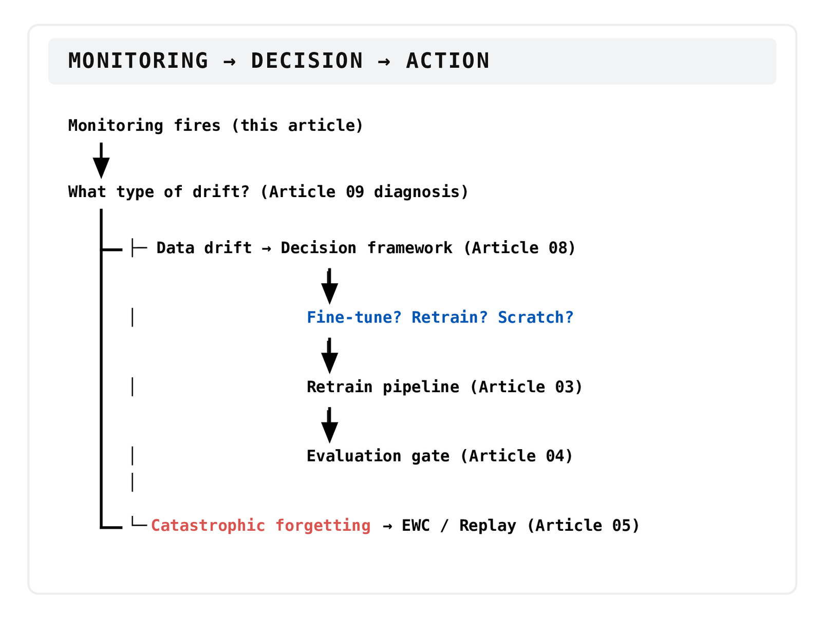
ML Model Monitoring: The Three Failure Modes That Look Identical From the Outside

Article 08 ended with a warning: before you retrain, diagnose. Three failure modes produce nearly identical symptoms — degraded performance on a production segment — but they require completely different responses.

Three Failure Modes — Same Symptom

Symptom: “Model is performing worse on segment X”

The monitoring stack in this article generates the evidence that routes you to the correct diagnosis. Without it, you are guessing.

Statistical Tests for Drift Detection: KS, PSI, and MMD

Three complementary statistical methods cover the full detection surface. They are complementary because each catches what the others miss.

Kolmogorov-Smirnov Test

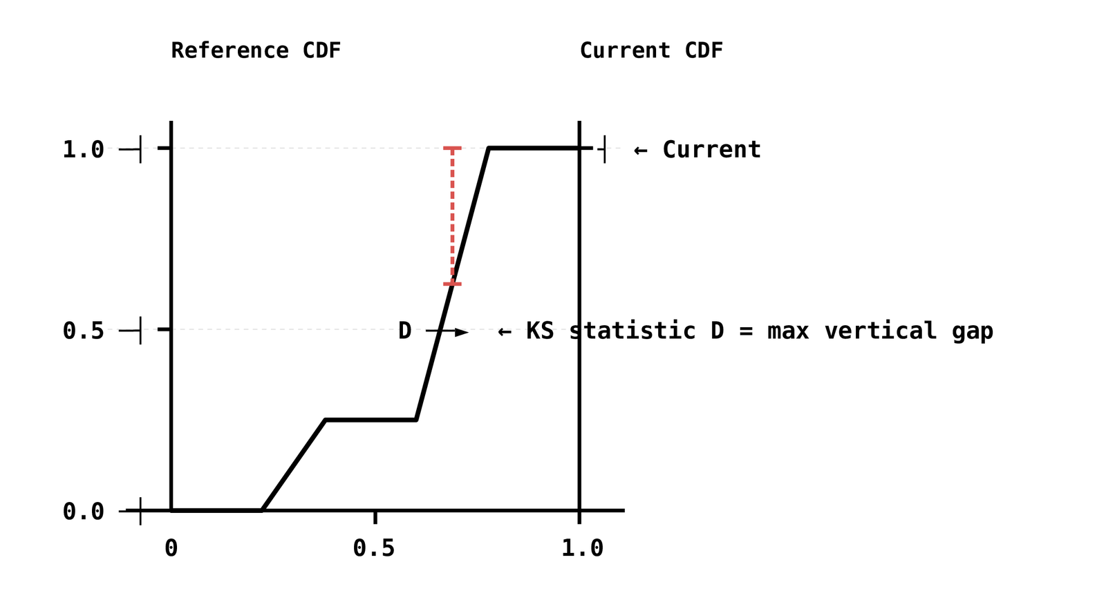
The KS test compares the empirical cumulative distribution functions (CDFs) of two samples and returns a test statistic D — the maximum vertical distance between the two CDFs — and a p-value.

When to use it: Per-feature marginal distribution checks. Run it on each input feature independently.

Thresholds:

• p ≥ 0.05 → stable, no action
• 0.01 ≤ p < 0.05 → warning, investigate
• p < 0.01 → critical, act

The implementation:

from detectors.statistical import KolmogorovSmirnovDetector

ks = KolmogorovSmirnovDetector(alpha=0.01)
results = ks.detect(reference_window, current_batch, feature_names)

for r in results:
    print(r)
# [DRIFT] KS  feature=transaction_amount  stat=0.2341  threshold=0.01  severity=critical
# [OK   ] KS  feature=merchant_category   stat=0.0412  threshold=0.01  severity=none

from detectors.statistical import KolmogorovSmirnovDetector

ks = KolmogorovSmirnovDetector(alpha=0.01)
results = ks.detect(reference_window, current_batch, feature_names)

for r in results:
    print(r)
# [DRIFT] KS  feature=transaction_amount  stat=0.2341  threshold=0.01  severity=critical
# [OK   ] KS  feature=merchant_category   stat=0.0412  threshold=0.01  severity=none

What KS misses: Joint distribution changes — cases where individual feature marginals look stable but correlations between features have shifted. A fraud model that uses 12 features may be vulnerable to a correlation shift that KS never detects on any single feature.

Population Stability Index (PSI)

PSI is the financial industry’s standard for model risk monitoring. It bins both distributions and computes a weighted log-ratio divergence.

Thresholds (industry standard):

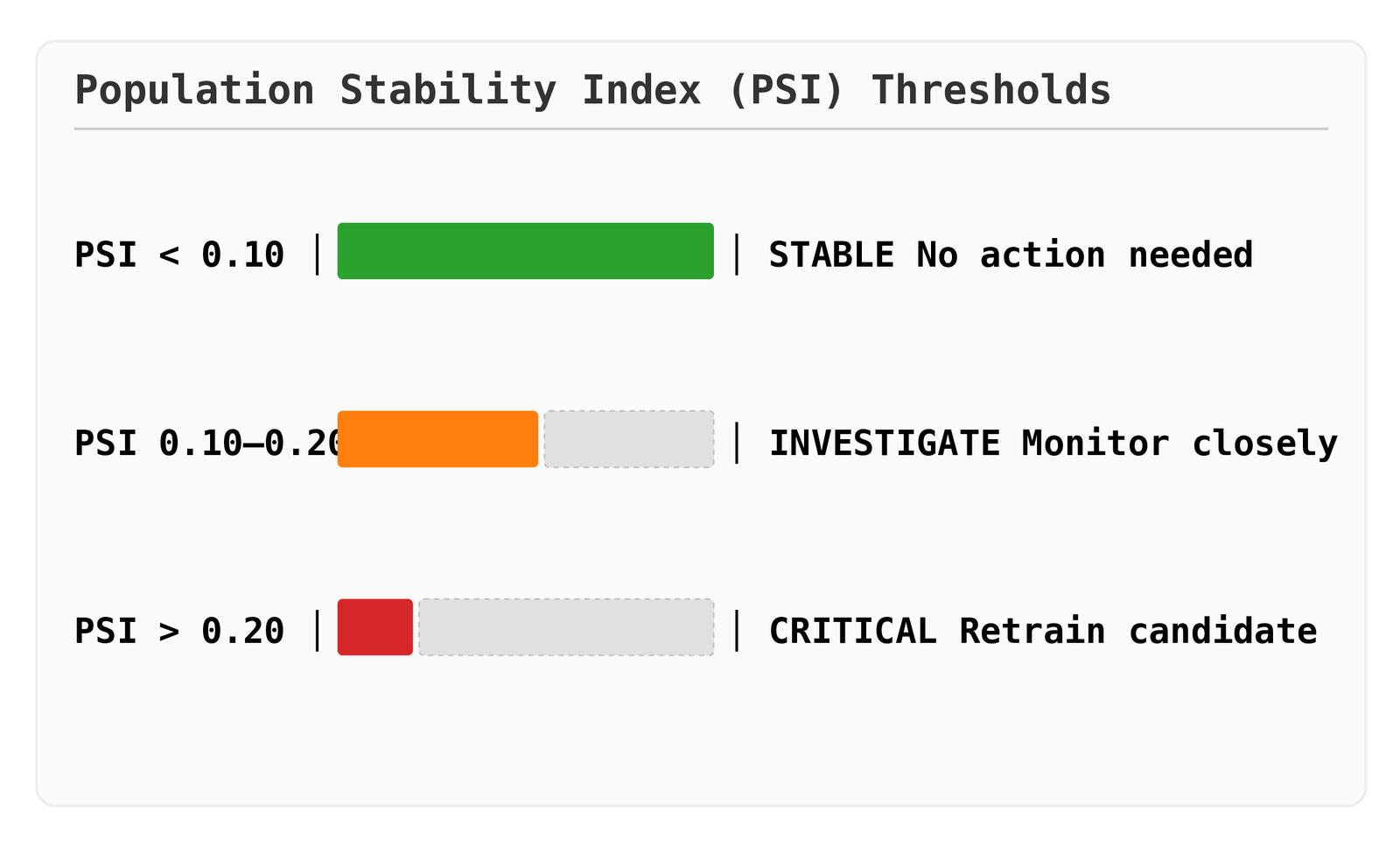
PSI has no p-value — it is a pure magnitude measure. That makes it easy to threshold but harder to interpret for small sample sizes where the magnitude can spike due to binning noise.

The benchmark output shows PSI fires fastest of all detectors across every scenario including the stable stream (Scenario A, batch 1). That is not a flaw — it is PSI’s known property: it fires on magnitude, not statistical significance. In production you pair PSI with KS. PSI catches everything early. KS confirms which detections are statistically significant.

from detectors.statistical import PopulationStabilityIndex

psi = PopulationStabilityIndex(n_bins=10)
results = psi.detect(reference_window, current_batch)

# PSI per feature
for r in results:
    if r.statistic > 0.20:
        alert(f"Critical PSI on {r.feature}: {r.statistic:.4f}")

from detectors.statistical import PopulationStabilityIndex

psi = PopulationStabilityIndex(n_bins=10)
results = psi.detect(reference_window, current_batch)

# PSI per feature
for r in results:
    if r.statistic > 0.20:
        alert(f"Critical PSI on {r.feature}: {r.statistic:.4f}")

Maximum Mean Discrepancy (MMD)

MMD tests whether two samples were drawn from the same distribution using a kernel (RBF in this implementation). Unlike KS and PSI, it operates on the joint feature distribution — it catches drift that individual feature marginals completely miss.

MMD uses a permutation test to compute its threshold. The observed MMD² statistic is compared to the null distribution built by randomly shuffling reference and current samples together. If the observed value exceeds the 95th percentile of the null distribution, drift is declared.

from detectors.statistical import MaximumMeanDiscrepancy

mmd = MaximumMeanDiscrepancy(alpha=0.05, n_permutations=100)
result = mmd.detect(reference_window, current_batch)

if result.drift_detected:
    print(f"Joint distribution drift: MMD²={result.statistic:.4f}, "
          f"p≈{result.p_value:.3f}")

from detectors.statistical import MaximumMeanDiscrepancy

mmd = MaximumMeanDiscrepancy(alpha=0.05, n_permutations=100)
result = mmd.detect(reference_window, current_batch)

if result.drift_detected:
    print(f"Joint distribution drift: MMD²={result.statistic:.4f}, "
          f"p≈{result.p_value:.3f}")

When to use it: When you suspect correlated drift — features that individually look stable but are shifting together. Catching fraud pattern changes is a canonical use case. Individual transaction amounts may be stable. Individual merchant category counts may be stable. But the correlation between amount and merchant that the model uses to detect fraud may have shifted significantly.

ADWIN and DDM: Sequential Drift Detectors

KS, PSI, and MMD are batch detectors — you call them with two windows of data. ADWIN and DDM are sequential detectors — they process one observation at a time and maintain no external windows.

ML Model Monitoring: ADWIN (ADaptive WINdowing)

ADWIN maintains an adaptive window of recent observations and continuously tests whether the left sub-window and the right sub-window have statistically different means. When the difference exceeds a Hoeffding-based threshold, the older half is discarded and a drift signal fires.

It requires no pre-specified window size. The window grows when the stream is stable and shrinks when drift occurs. This makes it robust to gradual drift where a fixed-window detector would average over the transition and miss it.

from detectors.adwin import ADWIN

adwin = ADWIN(delta=0.002)

for accuracy in rolling_accuracy_stream:
    if adwin.update(accuracy):
        print(f"ADWIN: drift detected at t={adwin.state().t}")
        trigger_retraining_pipeline()
        adwin.reset()

from detectors.adwin import ADWIN

adwin = ADWIN(delta=0.002)

for accuracy in rolling_accuracy_stream:
    if adwin.update(accuracy):
        print(f"ADWIN: drift detected at t={adwin.state().t}")
        trigger_retraining_pipeline()
        adwin.reset()

The delta parameter controls the false positive / detection delay trade-off. Lower delta → fewer false positives, higher detection delay. For production fraud detection, 0.002 is a reasonable default. For systems where fast response is critical, 0.005–0.01 is acceptable.

ML Model Monitoring: DDM (Drift Detection Method)

DDM monitors the model’s per-prediction error rate. It tracks the running error rate p and its standard deviation σ. When p + 2σ exceeds the minimum observed (p_min + 2σ_min), a warning fires. When p + 3σ exceeds it, drift is declared.

DDM is simpler than ADWIN and cheaper computationally. Its weakness is that it requires error labels — you need to know whether each prediction was correct, which means waiting for ground truth.

from detectors.ddm import DDM

ddm = DDM(warning_level=2.0, drift_level=3.0)

for is_error in error_stream:           # 1 = wrong, 0 = correct
    status = ddm.update(is_error)
    if status == "drift":
        retrain()
    elif status == "warning":
        start_collecting_new_data()

from detectors.ddm import DDM

ddm = DDM(warning_level=2.0, drift_level=3.0)

for is_error in error_stream:           # 1 = wrong, 0 = correct
    status = ddm.update(is_error)
    if status == "drift":
        retrain()
    elif status == "warning":
        start_collecting_new_data()

The benchmark result shows DDM missed every drift injection across all four scenarios. This is not a DDM failure — it is a ground truth latency problem. DDM needs to see the accumulation of errors over time, and with 200-sample batches and a clean test distribution, the signal takes longer to accumulate than the other detectors need. In production systems with delayed labels, DDM is most useful as a lagging confirmation signal rather than a first-line alert.

The Three Monitoring Layers in Code

Layer 1: Feature Monitor

from monitors.feature_monitor import FeatureMonitor

# Set from training distribution or first N production samples
monitor = FeatureMonitor(
    reference     = training_X,          # shape (n_ref, n_features)
    feature_names = feature_names,
    ks_alpha      = 0.01,
    rolling       = False,               # fixed reference window
)

# Call on each incoming batch
for batch in production_stream:
    report = monitor.update(batch.X)
    if report.any_drift:
        alert(f"Feature drift: {report.drifted_features_ks} (KS), "
              f"{report.drifted_features_psi} (PSI)")

from monitors.feature_monitor import FeatureMonitor

# Set from training distribution or first N production samples
monitor = FeatureMonitor(
    reference     = training_X,          # shape (n_ref, n_features)
    feature_names = feature_names,
    ks_alpha      = 0.01,
    rolling       = False,               # fixed reference window
)

# Call on each incoming batch
for batch in production_stream:
    report = monitor.update(batch.X)
    if report.any_drift:
        alert(f"Feature drift: {report.drifted_features_ks} (KS), "
              f"{report.drifted_features_psi} (PSI)")

Layer 2: Prediction Monitor

from monitors.prediction_monitor import PredictionMonitor

pred_monitor = PredictionMonitor(
    n_classes        = 3,
    reference_preds  = model.predict(training_X),
    reference_scores = model.predict_proba(training_X),
)

for batch in production_stream:
    preds  = model.predict(batch.X)
    scores = model.predict_proba(batch.X)
    report = pred_monitor.update(preds, scores)

    if report.label_shift_drift:
        alert("Label shift detected: class priors have changed")
    if report.confidence_drift:
        alert(f"Confidence distribution shift: mean={report.mean_confidence:.3f}")

from monitors.prediction_monitor import PredictionMonitor

pred_monitor = PredictionMonitor(
    n_classes        = 3,
    reference_preds  = model.predict(training_X),
    reference_scores = model.predict_proba(training_X),
)

for batch in production_stream:
    preds  = model.predict(batch.X)
    scores = model.predict_proba(batch.X)
    report = pred_monitor.update(preds, scores)

    if report.label_shift_drift:
        alert("Label shift detected: class priors have changed")
    if report.confidence_drift:
        alert(f"Confidence distribution shift: mean={report.mean_confidence:.3f}")

Layer 3: Performance Monitor

from monitors.performance_monitor import PerformanceMonitor

perf_monitor = PerformanceMonitor(
    n_classes     = 3,
    reference_acc = champion_accuracy,
    reference_f1  = champion_f1,
)

# When ground truth labels become available (may be delayed)
for batch in labelled_stream:
    report = perf_monitor.update(batch.y_true, batch.y_pred, batch.scores)
    if report.any_decay:
        alert(f"Performance decay: acc={report.accuracy:.4f} "
              f"(Δ{report.acc_delta:+.4f})")

from monitors.performance_monitor import PerformanceMonitor

perf_monitor = PerformanceMonitor(
    n_classes     = 3,
    reference_acc = champion_accuracy,
    reference_f1  = champion_f1,
)

# When ground truth labels become available (may be delayed)
for batch in labelled_stream:
    report = perf_monitor.update(batch.y_true, batch.y_pred, batch.scores)
    if report.any_decay:
        alert(f"Performance decay: acc={report.accuracy:.4f} "
              f"(Δ{report.acc_delta:+.4f})")

The Minimal Production Pipeline

Minimal ML Monitoring Pipeline (Production-Ready)

1. Log incoming features ← Every prediction request
2. Compare with reference window ← Batch or rolling window baseline
3. Compute PSI + KS per feature ← Batch job (every N samples)
4. Track prediction confidence ← Real-time (no labels required)
5. Evaluate with delayed labels ← When ground truth becomes available
6. Apply ADWIN on rolling accuracy ← Sequential detection (per prediction)
7. Trigger alert → route to diagnosis ← Avoid blind retraining

Step 7 routes to diagnosis, not immediately to retraining. The three failure modes in the table above require different responses. Acting before diagnosing compounds the failure — if the degradation is catastrophic forgetting from the last retraining cycle, triggering another retrain without replay makes it worse.

Head-to-Head Benchmark: Four Scenarios

All numbers below are from real runs. Seed: 42. Architecture: Nearest-Centroid classifier (intentionally naive — the article is about monitoring, not model choice). Device: CPU. Python 3.12. Total benchmark runtime: 50.4 seconds.

Scenario A — Stable Stream (No Drift)

The model is evaluated on 15 batches of 200 samples from the same distribution it was trained on. No drift injected.

Setup:
Champion trained on 1,000 samples
Evaluation stream: 15 batches × 200 = 3,000 samples

Interpretation:
Despite a high feature drift rate (73.3%), model performance remains perfect.
This highlights a critical point: not all data drift leads to model decay.

Reading these results honestly: PSI fires on 73.3% of batches on a stable stream. That is expected behavior — PSI is a magnitude measure and 200-sample batches have enough binning variance to push individual features over 0.10. ADWIN and DDM correctly produce zero false positives on the same stream.

This is the key lesson from Scenario A: PSI is a first-alert system, not a final verdict. In production, PSI > 0.10 should open an investigation, not trigger a retrain. Confirm with KS statistical significance before acting.

Scenario B — Abrupt Drift (shift_magnitude = 2.0)

Distribution shift injected at batch 5. All feature means shift by 2.0 standard deviations.

Setup:
True change point at batch 5
Evaluation performed on shifted distribution

Interpretation:
A sharp drop in accuracy and F1 confirms real performance degradation.
High feature drift (93.3%) aligns with the distribution shift.
ADWIN detects the change almost immediately, while DDM misses it, showing lower sensitivity to abrupt shifts.

A 42-percentage-point accuracy drop with a clean true change point at batch 5. ECE rising from 0.13 to 0.32 tells the second story: the model’s confidence scores are badly miscalibrated after the shift. It is still returning predictions with high confidence, but that confidence is wrong.

Scenario C — Gradual Drift (drift window: batches 4–9)

Mean shifts linearly from 0% to 100% displacement over batches 4 through 9. No sudden step.

Setup:
Drift begins at batch 4 and completes by batch 9
Evaluation performed across a progressively shifting distribution

Interpretation:
Performance degrades gradually, not abruptly, reflecting real-world drift patterns.
Although feature drift reaches 100%, the model adapts poorly over time, leading to steady accuracy loss.
ADWIN detects the change mid-drift (batch 7)—not at onset, but before total degradation.

ADWIN fires 3 batches after the drift onset. That detection delay is the cost of ADWIN’s robustness to noise — it needs to accumulate enough evidence to distinguish genuine drift from natural variance. For gradual drift in production, this delay is typically acceptable. The alternative — lowering delta to speed up detection — increases false positives on the stable stream.

Scenario D — Label Shift (class-0 prior: 33% → 70%)

Class 0 prevalence jumps from 33% to 70% at batch 5. Feature distributions for each class are unchanged — P(X|Y) is identical before and after.

Setup:
True change point at batch 5
Feature distributions remain unchanged (only label priors shift)

Interpretation:
Despite a major label distribution shift, model performance remains perfect.
However, feature drift signals fire incorrectly, creating a false alarm.
At the same time, ADWIN and DDM detect nothing, because predictions remain accurate.

This reveals a critical gap:
standard monitoring pipelines can both overreact and miss real distribution changes simultaneously.

Accuracy stays at 1.0. F1 stays at 1.0. ADWIN and DDM produce zero detections. Feature drift rate is 93.3% — but that is a false signal caused by the shifted class composition changing the marginal feature distributions.

A team relying only on accuracy monitoring would see nothing wrong. A team relying only on feature monitoring would see noise. A team relying on prediction distribution monitoring would catch this: the chi-squared test on class counts detects the prior shift at batch 6 — one batch after the true change point.

Label shift matters even when current performance is fine, because the model’s calibration assumptions have changed. A model calibrated on a balanced dataset is now seeing class 0 70% of the time. Its posterior probability estimates are wrong relative to the new prior. If this model is used to make threshold-based decisions, those thresholds need recalibration.

Detector Comparison: First Detection Batch

Ground truth change point (CP) is shown for reference.
Detection timing is reported as the first batch where the detector fired.

Key:

• b.N → First detection at batch N
• missed → No detection triggered

No single detector wins across all scenarios. PSI is fastest but noisiest. KS is more precise but slower on gradual changes. MMD catches joint distribution changes that per-feature tests miss. ADWIN reliably catches performance impact but requires more evidence to fire. DDM needs longer accumulation than the benchmark’s 15-batch window allows.

Production recommendation: run PSI + KS as the primary alert layer. Use MMD monthly for deep correlation audits. Use ADWIN on rolling accuracy as the ground-truth performance layer.

Real-World Failure Scenario: The Fraud Model That Looked Fine

A fraud detection model is trained on transaction data from Q1 2024. It reaches 94% accuracy on the held-out test set and gets deployed.

By Q3 2024:

• Buy-now-pay-later services have grown from 3% to 19% of transactions in the user base
• Average transaction size has shifted from $47 median to $83 median
• The correlation between transaction hour and fraud probability has changed as mobile usage patterns shift

What the monitoring dashboard shows: 95.2% accuracy. No alerts.

What is actually happening: The model has never seen the BNPL transaction pattern. It classifies those confidently — but wrong. ECE has climbed from 0.04 to 0.17, meaning its confidence estimates are significantly miscalibrated. The actual fraud detection rate on BNPL transactions is 41%, not the reported 95%.

What would have caught it:

• PSI > 0.25 on payment_method feature: would have fired in week 2 of Q2
• MMD on joint distribution: would have fired in week 4 of Q2
• ECE monitoring: would have shown calibration degradation in week 3 of Q2

The ground truth accuracy metric was masked by the majority of transactions still being traditional card payments where the model still works well. Aggregate accuracy hides slice-level failure.

How to Set Detection Thresholds in Practice

The right thresholds depend on how fast your domain moves and what a missed detection costs. These are starting points, not universal rules.

THRESHOLD GUIDE BY METRIC

KS test p-value
  p ≥ 0.05   →  Stable. No action.
  0.01–0.05  →  Warning. Monitor closely. Check PSI.
  p < 0.01   →  Critical. Confirm with MMD. Route to Article 09 diagnosis.

PSI per feature
  < 0.10     →  Stable.
  0.10–0.20  →  Investigation zone. PSI alone is not enough.
  > 0.20     →  Significant. Act if KS also fires. Retrain candidate.
  > 0.25     →  Emergency. Immediate investigation.

ECE (Expected Calibration Error)
  < 0.05     →  Well calibrated.
  0.05–0.10  →  Acceptable for most use cases.
  > 0.10     →  Confidence scores unreliable. Threshold decisions at risk.
  > 0.20     →  Severely miscalibrated. Confidence outputs should not be used.

ADWIN delta parameter
  0.002      →  Conservative. Low false positives. Higher detection latency.
  0.005      →  Balanced. Recommended starting point.
  0.01       →  Aggressive. Fast detection. Higher false positive rate.

One rule that overrides all thresholds: never retrain without an evaluation gate. Article 03 built the retraining pipeline. Article 08 built the decision framework for what strategy to use. This article provides the signals that trigger those systems. The three pieces connect: detect (here) → decide (Article 08) → retrain (Article 03) → gate (Article 04).

Code: PSI From Scratch

The full PSI implementation used in this benchmark:

import numpy as np

def psi(reference: np.ndarray, current: np.ndarray,
        n_bins: int = 10, epsilon: float = 1e-4) -> float:
    """
    Population Stability Index for a 1-D feature.

    Returns
    -------
    float
        PSI value. < 0.10: stable | 0.10-0.20: investigate | > 0.20: critical
    """
    combined = np.concatenate([reference, current])
    bins = np.linspace(combined.min(), combined.max(), n_bins + 1)
    bins[0], bins[-1] = -np.inf, np.inf

    ref_pct = np.histogram(reference, bins=bins)[0] / len(reference) + epsilon
    cur_pct = np.histogram(current,   bins=bins)[0] / len(current)   + epsilon

    ref_pct /= ref_pct.sum()
    cur_pct /= cur_pct.sum()

    return float(np.sum((cur_pct - ref_pct) * np.log(cur_pct / ref_pct)))


# Usage
psi_value = psi(training_feature, production_feature)

if psi_value > 0.20:
    print(f"Critical drift: PSI={psi_value:.4f}")
elif psi_value > 0.10:
    print(f"Warning: PSI={psi_value:.4f}. Investigate.")
else:
    print(f"Stable: PSI={psi_value:.4f}")

import numpy as np

def psi(reference: np.ndarray, current: np.ndarray,
        n_bins: int = 10, epsilon: float = 1e-4) -> float:
    """
    Population Stability Index for a 1-D feature.

    Returns
    -------
    float
        PSI value. < 0.10: stable | 0.10-0.20: investigate | > 0.20: critical
    """
    combined = np.concatenate([reference, current])
    bins = np.linspace(combined.min(), combined.max(), n_bins + 1)
    bins[0], bins[-1] = -np.inf, np.inf

    ref_pct = np.histogram(reference, bins=bins)[0] / len(reference) + epsilon
    cur_pct = np.histogram(current,   bins=bins)[0] / len(current)   + epsilon

    ref_pct /= ref_pct.sum()
    cur_pct /= cur_pct.sum()

    return float(np.sum((cur_pct - ref_pct) * np.log(cur_pct / ref_pct)))


# Usage
psi_value = psi(training_feature, production_feature)

if psi_value > 0.20:
    print(f"Critical drift: PSI={psi_value:.4f}")
elif psi_value > 0.10:
    print(f"Warning: PSI={psi_value:.4f}. Investigate.")
else:
    print(f"Stable: PSI={psi_value:.4f}")

How Often Should You Monitor? Heuristics by Domain

There is no universal monitoring cadence. The right answer depends on how fast your data distribution moves and how expensive a missed detection is.

Different applications require different monitoring frequencies based on how fast data changes and how quickly ground truth becomes available.

One rule holds across all domains: monitoring cadence should match data velocity, not your deployment schedule. A model deployed quarterly that processes real-time transactions needs hourly monitoring regardless of retraining frequency.

Transfer Learning vs Continual Learning vs Monitoring: Where This Fits

Article 07 established three continual learning scenarios. Article 08 gave the decision framework for when to retrain vs fine-tune. This article provides the signal layer that feeds those decisions.

A drift alert is not a retrain command. It is the beginning of a diagnosis workflow. Skipping diagnosis and going straight to retrain is the most common and most expensive mistake teams make.

FAQ

Key Takeaways

• ML models fail silently. Accuracy alone is a lagging, aggregate metric that hides slice-level failure.
• Data drift affects inputs and is measurable without ground truth labels. Model decay affects outcomes and requires labels to confirm.
• PSI > 0.2 on any input feature is a strong signal. Confirm with KS before acting.
• ECE climbing above 0.10 means your model’s confidence outputs are unreliable for threshold-based decisions.
• No single detector covers the full failure surface. PSI + KS + MMD + ADWIN is the minimum production stack.
• Label shift (Scenario D) produces 93.3% feature drift alerts and zero performance degradation simultaneously. Monitoring without a prediction layer will misdiagnose this every time.
• A drift alert is a diagnosis trigger, not a retrain command. Route to the Article 08 decision framework before acting.
• Never retrain without an evaluation gate. A challenger that improves on the new distribution while degrading on the old one is not an improvement.

What Is Next

This article opens Cluster 3. Articles 09–12 together form the complete monitoring and observability stack: detecting drift (this article), building a Streamlit dashboard (Article 10), shadow deployment and canary testing (Article 11), and debugging latency and throughput in ML inference (Article 12).

Article 10 — How to Build an ML Monitoring Dashboard from Scratch (Streamlit Tutorial) builds the visual layer on top of the monitors built here. The FeatureMonitor, PredictionMonitor, and PerformanceMonitor objects from this codebase connect directly to the Streamlit interface in Article 10. The detectors do not change — only the visualization layer.

If your model is already degrading and you need to diagnose the failure mode before building a full monitoring stack, this article’s benchmark scenarios and the three-failure-mode table are the right starting point.

Complete code: https://github.com/Emmimal/ML-Model-Monitoring

References

[1] Gama, J., Žliobaitė, I., Bifet, A., Pechenizkiy, M., & Bouchachia, A. (2014). A survey on concept drift adaptation. ACM Computing Surveys, 46(4), Article 44. https://doi.org/10.1145/2523813

[2] Bifet, A., & Gavalda, R. (2007). Learning from time-changing data with adaptive windowing. In Proceedings of the 2007 SIAM International Conference on Data Mining (pp. 443–448). https://doi.org/10.1137/1.9781611972771.42

[3] Gretton, A., Borgwardt, K. M., Rasch, M. J., Schölkopf, B., & Smola, A. (2012). A kernel two-sample test. Journal of Machine Learning Research, 13, 723–773. http://jmlr.org/papers/v13/gretton12a.html

[4] Massey, F. J. (1951). The Kolmogorov-Smirnov test for goodness of fit. Journal of the American Statistical Association, 46(253), 68–78. https://www.tandfonline.com/doi/abs/10.1080/01621459.1951.10500769

[5] Yurdakul, Bilal & Naranjo, Joshua. (2020). Statistical Properties of the Population Stability Index. Journal of Risk Model Validation. 10.21314/JRMV.2020.227.

[6] Guo, C., Pleiss, G., Sun, Y., & Weinberger, K. Q. (2017). On calibration of modern neural networks. Proceedings of the 34th International Conference on Machine Learning (ICML). https://doi.org/10.48550/arXiv.1706.04599

[7] Gama, J., Medas, P., Castillo, G., & Rodrigues, P. (2004). Learning with drift detection. In Brazilian Symposium on Artificial Intelligence (pp. 286–295). Springer.

[8] Baena-García, M., del Campo-Ávila, J., Fidalgo, R., Bifet, A., Gavalda, R., & Morales-Bueno, R. (2006). Early drift detection method. In 4th ECML PKDD International Workshop on Knowledge Discovery from Data Streams.

[9] Pedregosa, F., Varoquaux, G., Gramfort, A., Michel, V., Thirion, B., Grisel, O., … & Duchesnay, E. (2011). Scikit-learn: Machine learning in Python. Journal of Machine Learning Research, 12, 2825–2830. http://jmlr.org/papers/v12/pedregosa11a.html

[10] Virtanen, P., Gommers, R., Oliphant, T. E., Haberland, M., Reddy, T., Cournapeau, D., … & SciPy 1.0 Contributors. (2020). SciPy 1.0: Fundamental algorithms for scientific computing in Python. Nature Methods, 17, 261–272. https://doi.org/10.1038/s41592-020-0772-5

Disclosure

Code authorship: All code in this article — the five stream generators (StableStreamGenerator, AbruptDriftGenerator, GradualDriftGenerator, SeasonalDriftGenerator, LabelShiftGenerator); the three statistical detectors (KolmogorovSmirnovDetector, PopulationStabilityIndex, MaximumMeanDiscrepancy); the two sequential detectors (ADWIN, DDM + EDDM); the three monitor classes (FeatureMonitor, PredictionMonitor, PerformanceMonitor); the MonitoringMetrics and DetectorComparisonResult dataclasses; the four-scenario benchmark runner; and the 32-test unit suite — is the original work of the author. The framework builds on NumPy [Harris et al., 2020], SciPy [10], and scikit-learn [9], all open-source under BSD licenses.

Benchmark authenticity: All benchmark numbers in this article are from real runs executed by the author on CPU (Python 3.12, NumPy 1.24+, SciPy 1.10+, scikit-learn 1.3+). Seed: 42. The output shown matches logged output verbatim. No numbers were adjusted or estimated. Total benchmark runtime: 50.4 seconds.

Dataset: All experiments use synthetic Gaussian mixture datasets generated programmatically in data/generators.py. No external dataset downloads are required.

No affiliate relationships: No tools, libraries, or services are mentioned for compensation. All recommendations reflect independent technical evaluation. All referenced tools are open-source under MIT or BSD licenses.

Series affiliation: This is Article 09 of the Production ML Engineering series published at EmiTechLogic. Articles 01–08 are linked throughout where referenced.

Series: Production ML Engineering — Article 09 of 15 Previous: Retrain vs Fine-Tune vs Train from Scratch: A Decision Framework for ML Engineers (Article 08) Next: ML Monitoring Dashboard with Streamlit (Article 10) Hub: Production ML Engineering Guide (Article 01)