

Retrain vs Fine-Tune vs Train from Scratch: A Decision Framework for ML Engineers
When dealing with production ML systems, the decision between Retrain vs Fine-Tune is rarely straightforward. Most teams choose based on habit rather than measurable signals, leading to unnecessary compute cost or degraded performance in production.
Series: Production ML Engineering — Article 08 of 15 (Cluster 2: Continual Learning)
Before you read this: This article is part of a 15-part series on building production-grade ML systems. If you have not read the series hub yet, start with the Production ML Engineering guide — it maps out the five pillars every production system rests on. Articles 02–04 covered deployment, retraining pipelines, and model versioning. Articles 05–07 covered catastrophic forgetting, online learning, and the three continual learning scenarios. This article closes Cluster 2 with the decision that comes before all of them: which strategy do you actually use, and when?
The drift monitor fires. New labelled data arrives. Then someone asks: “Are we retraining or fine-tuning?”
Most teams answer based on habit. The team that retrains every month keeps retraining. The team that read a transfer learning tutorial fine-tunes everything. Nobody has a real argument for why.
That gap is expensive.
Choosing fine-tuning when the distribution has shifted severely gives you a model that moves its decision boundary while the underlying representations stay wrong. Choosing full retraining when you only have 200 target-domain samples gives you a model that never converges properly.
The worst part? The mistake does not always show up in your evaluation metrics right away. It shows up three weeks later when a segment of predictions that looked fine in testing quietly falls apart in production.
This article documents the decision framework I use in production. Three strategies. Four real-world scenarios. A head-to-head benchmark with exact numbers from real runs. And a rule-based decision engine that maps observable signals to a recommendation.
Everything is code-first. All numbers are from real runs.
Complete Code: https://github.com/Emmimal/Retrain-vs-Fine-Tune/
Why Getting This Decision Wrong Is Expensive
Every strategy choice carries a cost across three dimensions.
Compute cost is proportional to how many parameters you update and for how many gradient steps. Head-only fine-tuning updates around 512 parameters. Full retraining updates 267,000. That is not a 1.5x difference. It is over 500x, as the cost model in this article shows.
Forgetting cost is the accuracy drop on tasks the model already knew. Article 05 documented how gradient interference destroys prior knowledge when nothing constrains it. The strategy you choose directly controls whether that destruction happens. Kirkpatrick et al. [4] showed that unconstrained gradient updates during sequential training can catastrophically overwrite prior task knowledge — the strategy you choose is the primary control over whether that occurs.
Data cost is how much labelled data the strategy needs to converge. Training from scratch on 200 examples does not converge. Fine-tuning a good trunk on 200 examples does. The minimum viable dataset size is not fixed — it depends on how much prior knowledge the strategy preserves.
These three dimensions pull against each other. There is no dominant strategy. There is only the right strategy for the signals in front of you.
What Is Fine-Tuning in Machine Learning?
Fine-tuning starts from a pre-trained model’s weights and updates some or all of them on new data. No re-initialisation. Prior training is a warm start.
Two variants matter in production, and the choice between them is a second-order decision that is just as important as the first-order choice between fine-tuning and retraining.
Head-only fine-tuning (frozen trunk): The shared feature extractor — everything except the final linear layer — is frozen. Only the output head is trainable. This is the lowest-cost strategy: one linear layer, a few epochs, and the trunk representations cannot be destroyed because the trunk weights are physically immutable during training.
Full fine-tuning (unfrozen trunk): All parameters are trainable, but at a lower learning rate than initial training — typically 10x lower. The trunk can adapt to the new distribution, at the cost of potentially overwriting prior representations. Howard and Ruder [3] established this lower-learning-rate discipline as a core practice for effective fine-tuning — training at the original learning rate risks destroying the representations the trunk already learned.
from strategies.fine_tune import FineTuner, FineTuneMode

# Head-only: trunk frozen, only the output layer trains
tuner  = FineTuner(model, mode=FineTuneMode.HEAD_ONLY, epochs=10, lr=0.01)
result = tuner.fine_tune(new_data_loader)

# Full fine-tune: all parameters trainable, 10x lower LR
tuner  = FineTuner(model, mode=FineTuneMode.FULL_NETWORK, epochs=10, lr=0.001)
result = tuner.fine_tune(new_data_loader)The above code uses PyTorch [8], an open-source deep learning library under the BSD license. The freeze_trunk() implementation in models/base_model.py is explicit:
def freeze_trunk(self) -> None:
    """Freeze trunk; head remains trainable (standard fine-tuning)."""
    for param in self.trunk.parameters():
param.requires_grad = FalseOne design detail worth noting: after fine_tune() returns, unfreeze_trunk() is called automatically. The model is always in a clean state for whatever comes next, regardless of which mode ran.
What Is Model Retraining? (And When Is It Different from Fine-Tuning?)
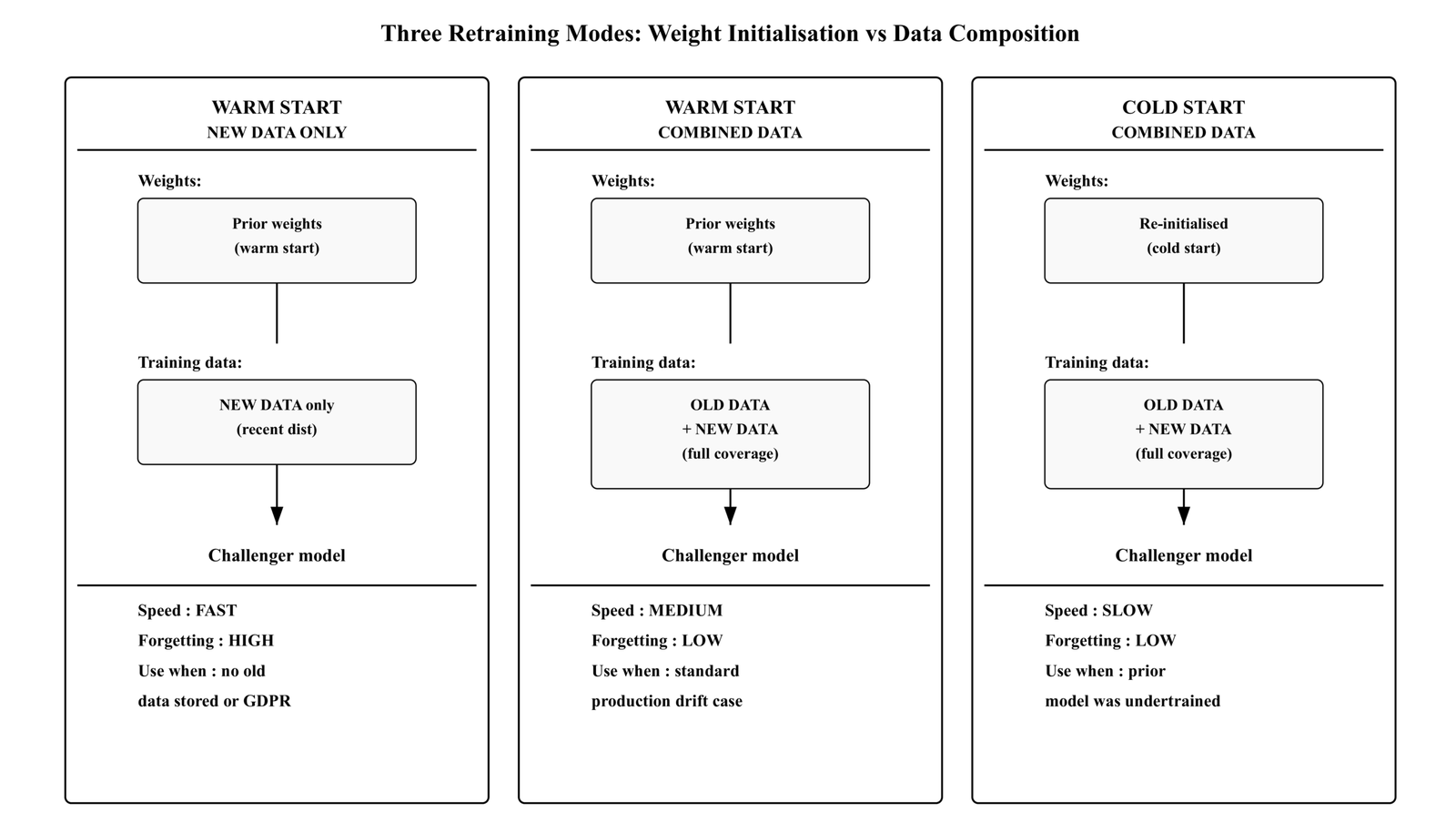
Retraining also starts from prior weights — a warm start — but trains on a dataset that includes data from previous windows. Three modes matter:
Warm start, new data only: Prior weights as the starting point. Training data is the new distribution only. Faster convergence than scratch, but the same forgetting risk as unconstrained full fine-tuning.
Warm start, combined data: Prior weights. Old data plus new data together. This is the standard production retraining approach for gradual drift. It adapts to new patterns while keeping prior distribution examples alive in the gradient signal.
Cold start, combined data: Weights re-initialised. Old plus new data. Equivalent to training from scratch on the full combined dataset. Use this when the prior model was severely undertrained or when there is evidence the warm start is actively harmful.
from strategies.retrain import Retrainer, RetrainMode

# Standard production case: warm start on combined data
retrainer = Retrainer(model, mode=RetrainMode.WARM_COMBINED, lr=0.005, epochs=10)
result    = retrainer.retrain(new_loader, old_loader=old_loader)

# Fast update: warm start, new data only (higher forgetting risk)
retrainer = Retrainer(model, mode=RetrainMode.WARM_NEW_ONLY, lr=0.005, epochs=10)
result = retrainer.retrain(new_loader)The key difference from fine-tuning is data composition, not weight initialisation. Retraining is the answer when you have retained historical data and need to preserve prior distribution coverage while adapting to the new one. Fine-tuning is the answer when historical data is unavailable, unnecessary, or prohibited by policy.
Signs Your Model Needs Retraining
These are the production signals that should trigger a strategy decision, in order of urgency. Drift detectors such as ADWIN and DDM are grounded in the concept drift adaptation literature [7]:
Production Signals & Strategy Triggers
| Signal | Urgency | Action / Description |
| Drift detector fires (ADWIN/DDM) | Act within 24 hours | Immediate investigation into data or concept drift. |
| Champion accuracy drops > 5% | Evaluate within 48 hours | Assess model performance degradation against baselines. |
| New labelled data batch arrives | Schedule update | Queue the data for the next routine model retraining cycle. |
| New output classes introduced | Architecture decision | Requires structural changes to the model and deployment pipeline. |
| Data retention window expires | Use new data only | Enforce compliance and privacy by purging old training data. |
| Stakeholder flags segment failure | Diagnose first (Art. 09) | Initiate targeted slice analysis before taking corrective action. |
One rule holds before you act on any of these: drift detector fires ≠ immediately retrain.
First diagnose whether the degradation is concept drift, data drift, or catastrophic forgetting from a prior retraining cycle [7]. Article 09 covers this in detail. Acting on the wrong diagnosis with the wrong strategy compounds the failure.
The Decision Tree: Retrain, Fine-Tune, or Start Over?
The decision engine in evaluation/decision_framework.py makes these rules explicit. Every recommendation traces back to a specific signal.
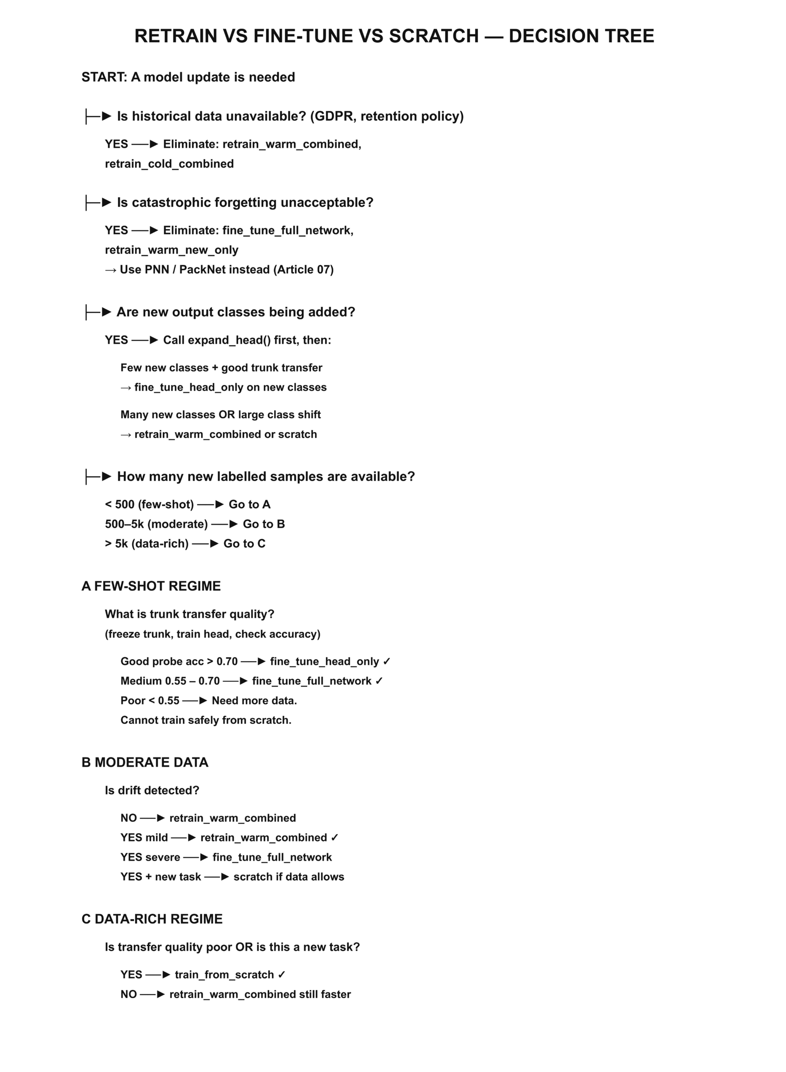
Here is how you use the decision engine directly:
from evaluation.decision_framework import (
    DataSignals, ModelSignals, DriftSignals,
    ConstraintSignals, DecisionEngine,
)

engine = DecisionEngine()
result = engine.decide(
    data        = DataSignals(
        n_new_samples        = 300,
        n_historical_samples = 1_000,
    ),
    model       = ModelSignals(
        current_accuracy     = 0.94,
        accuracy_on_new_data = 0.72,
        transfer_quality     = 0.76,
    ),
    drift       = DriftSignals(
        drift_detected = True,
        drift_severity = "moderate",
    ),
    constraints = ConstraintSignals(
        can_store_historical = True,
    ),
)
print(result.summary())Output:
======================================================================
  DECISION ENGINE OUTPUT
======================================================================

PRIMARY RECOMMENDATION
----------------------------------------------------------------------
  Strategy   : retrain_warm_combined
  Confidence : high
  Rationale  : Drift detected with historical data available.
               Warm-start combined training is the standard production
               response — adapts to new data while retaining
               old distribution coverage.
======================================================================
Head-to-Head Benchmark
All numbers are from real runs. Seed: 42. Architecture: MLP [128, 64]. Device: CPU. Python 3.12, PyTorch 2.0+ [8]. Total benchmark runtime: 13.4 seconds.
Scenario A — New Data, Same Distribution
Champion trained on 1,000 samples. Update adds 500 same-distribution samples. Test on the same distribution.
SCENARIO A — New Data, Same Distribution Champion: 1,000 samples | Update: +500 same-dist | Test: 400 samples
| Strategy | ACC | F1 | ECE | Time |
| Champion (no update) | 0.9775 | 0.9775 | 0.0163 | 0.00s |
| FineTune head-only | 0.9775 | 0.9775 | 0.0183 | 0.12s |
| FineTune full network | 0.9750 | 0.9750 | 0.0128 | 0.22s |
| Retrain warm new-only | 0.9750 | 0.9750 | 0.0234 | 0.22s |
| Retrain warm combined | 0.9700 | 0.9700 | 0.0200 | 0.64s |
| Retrain cold combined | 0.9775 | 0.9775 | 0.0206 | 0.98s |
| Scratch (combined) | 0.9675 | 0.9675 | 0.0268 | 0.96s |
Reading these results honestly: every strategy clusters within 1% of the champion. The distribution is stable and performance is already near the ceiling.
No strategy produces a meaningful accuracy gain. The decision here is cost, not performance.
Head-only fine-tuning matches the champion at 0.12 seconds. Retrain cold combined costs 0.98 seconds for the exact same accuracy. Scratch is the worst performer while being one of the most expensive options.
This is the most common production scenario. And it is the one teams spend the most time overthinking. When the distribution is stable and performance is already high, pick the lowest-cost option that does not increase forgetting risk. That is head-only fine-tuning.
Scenario B — Distribution Shift
Champion trained on the original distribution. Update data is from a shifted distribution (shift_magnitude=1.5). Test set is drawn from the shifted distribution only.
SCENARIO B — Distribution Shift (shift_magnitude=1.5) Champion: original distribution | Test: SHIFTED distribution only
| Strategy | ACC | F1 | ECE | Time |
| Champion (no update) | 0.5000 | 0.3333 | 0.5000 | 0.00s ← chance |
| FineTune head-only | 0.9925 | 0.9925 | 0.0138 | 0.15s ← winner |
| FineTune full network | 0.9925 | 0.9925 | 0.0103 | 0.27s |
| Retrain warm combined | 0.8550 | 0.8519 | 0.0330 | 0.77s |
| Scratch (shifted data) | 0.9775 | 0.9775 | 0.0170 | 0.33s |
Reading these results honestly: the champion at 0.5000 is performing at chance. The distribution moved far enough that the original decision boundary is useless.
Head-only fine-tuning recovers to 0.9925 in 0.15 seconds. That seems counterintuitive — if the distribution shifted, why does freezing the trunk work?
The trunk learns general feature representations — directions in the input space that are predictive. Yosinski et al. [2] demonstrated that lower-level network features transfer well across tasks and domains; a shift in class means does not destroy those representations. It moves where the decision boundary should sit. The head is the boundary. Head-only fine-tuning updates exactly the right layer.
Retrain warm combined at 0.8550 is the worst performer after the unmodified champion. Including old distribution data during training creates a tug-of-war. The old data pulls weights back toward the prior boundary. The new data pulls them toward the shifted one. When the test set is exclusively the new distribution, that conflict hurts.
Scenario C — New Classes
Champion trained on 3-class task. Update introduces 2 new classes. Test covers all 5 classes. Old-class accuracy and new-class accuracy are reported separately.
SCENARIO C — New Classes (3 original → 5 total) Test: all 5 classes | 300 samples per class
| Strategy | ACC | F1 | ECE | Time | Old acc | New acc |
| Expand + head-only FT | 0.3980 | 0.2784 | 0.6049 | 0.17s | — | 0.995 |
| Expand + full FT (combined) | 0.9860 | 0.9860 | 0.0674 | 0.73s | 0.987 | 0.985 |
| Retrain warm combined | 0.9900 | 0.9900 | 0.0178 | 0.92s | 0.987 | 0.995 |
| Scratch (all 5 classes) | 0.9920 | 0.9920 | 0.0180 | 1.37s | 0.990 | 0.995 |
Reading these results honestly: head-only expansion is a specific failure mode that is easy to miss.
New-class accuracy is 0.995 — the head learned the new classes perfectly. Old-class accuracy is near zero. Overall accuracy collapses to 0.3980.
Here is what happened. The frozen trunk has never seen the new class distributions. New-class examples land in unpredictable regions of the feature space. The old head weights that classified correctly before are now being used by the expanded head for a completely different purpose. The head cannot compensate for a trunk that has no information about the new classes.
Head-only expansion with new-class data only works when you have both old and new class data in the training set simultaneously, so the expanded head can learn the joint decision boundary. Without old class examples in the training loop, the head has no way to separate new from old.
Full fine-tuning on combined data (0.9860) and retrain warm combined (0.9900) both solve this correctly. For most production deployments, retrain warm combined is the right default.
Scenario D — Domain Transfer
Model pre-trained on 2,000 source-domain samples. Target domain has 200 labelled examples and a domain shift of 2.0. Test on the target distribution.
SCENARIO D — Domain Transfer (few-shot target) Pre-trained: 2,000 source samples | Target: 200 samples | shift=2.0
| Strategy | ACC | F1 | ECE | Time |
| Source model (no FT) | 0.3333 | 0.1702 | 0.6586 | 0.00s ← useless |
| FineTune head-only | 0.9424 | 0.9425 | 0.0186 | 0.13s ← winner |
| FineTune full network | 0.9474 | 0.9473 | 0.0352 | 0.24s |
| Scratch (200 target) | 0.8797 | 0.8804 | 0.0803 | 0.32s |
Reading these results honestly: this is the clearest argument for fine-tuning in the entire benchmark.
Scratch on 200 samples reaches 0.8797. Head-only fine-tuning from the source-pretrained model reaches 0.9424 with the exact same data. A 6.3 percentage point gain, at 0.13 seconds versus 0.32 seconds.
The source trunk provides representations that generalise to the target domain even though the surface statistics differ [1, 9]. Training from scratch throws away that advantage entirely.
The ECE numbers make a second point. Scratch at 0.0803 is poorly calibrated — the model is overconfident on a task with too little training data. Head-only fine-tuning at 0.0186 is well calibrated because the trunk’s uncertainty estimates are already reliable and only the head needed to adapt.
How Often Should You Retrain? (Practical Heuristics by Industry)
There is no universal frequency. The right cadence depends on how fast your data distribution moves and what a stale model actually costs you.
RETRAINING FREQUENCY HEURISTICS BY DOMAIN
| Domain | Typical Cadence | Trigger Type |
|---|---|---|
| Fraud detection | Daily–weekly | Drift-based |
| Recommendation systems | Hours–daily | Online (Art. 06) |
| NLP classifiers | Monthly–quarterly | New domain data |
| Medical imaging | Quarterly+ | Annotated batch |
| Financial forecasting | Daily | Market regime |
| Content moderation | Weekly | Policy + drift |
| Industrial sensors | Monthly | Equipment cycle |
The right framework is not a calendar. It is a trigger. Article 03 built the retraining pipeline. Article 06 built the drift detectors. Those two systems tell you when to act. This article tells you what to do when they fire.
One rule holds across all domains: never retrain without an evaluation gate. The challenger must beat or match the champion on both the new distribution and the prior distribution before promotion. A challenger that improves on new data while forgetting old data is not an improvement.
Transfer Learning vs Continual Learning: What Is the Difference?
This comes up in every team that has read both transfer learning tutorials and continual learning papers, and it matters for strategy selection.
Transfer learning [1, 9] uses a pre-trained model as an initialisation point for a new target task. Once transfer is complete, prior task performance is irrelevant. You do not measure whether the fine-tuned model still performs on ImageNet.
Continual learning [5] (Articles 05–07) requires the model to perform well on all tasks it has ever seen, simultaneously. Forgetting any prior task is a failure.
TRANSFER LEARNING vs CONTINUAL LEARNING
| You need the updated model to… | Use… |
|---|---|
| Perform well on the new task only | Transfer learning |
| (prior task performance irrelevant) | (this article) |
| Perform well on ALL tasks simultaneously | Continual learning |
| (any forgetting is a failure) | (Articles 05 + 07) |
| Adapt to a continuous stream of data | Online learning |
| (no discrete task boundaries) | (Article 06) |
Most production retraining problems are transfer learning problems in disguise.
The fraud model from six months ago does not need to still classify fraud from six months ago. It needs to classify fraud from today. That is not continual learning. It is fine-tuning or retraining on a shifted distribution, and the methods in this article apply directly.
Cost Model: What Each Strategy Costs Over a Model’s Lifetime
The benchmark runtimes above are per update. The lifetime cost is what matters for production planning.
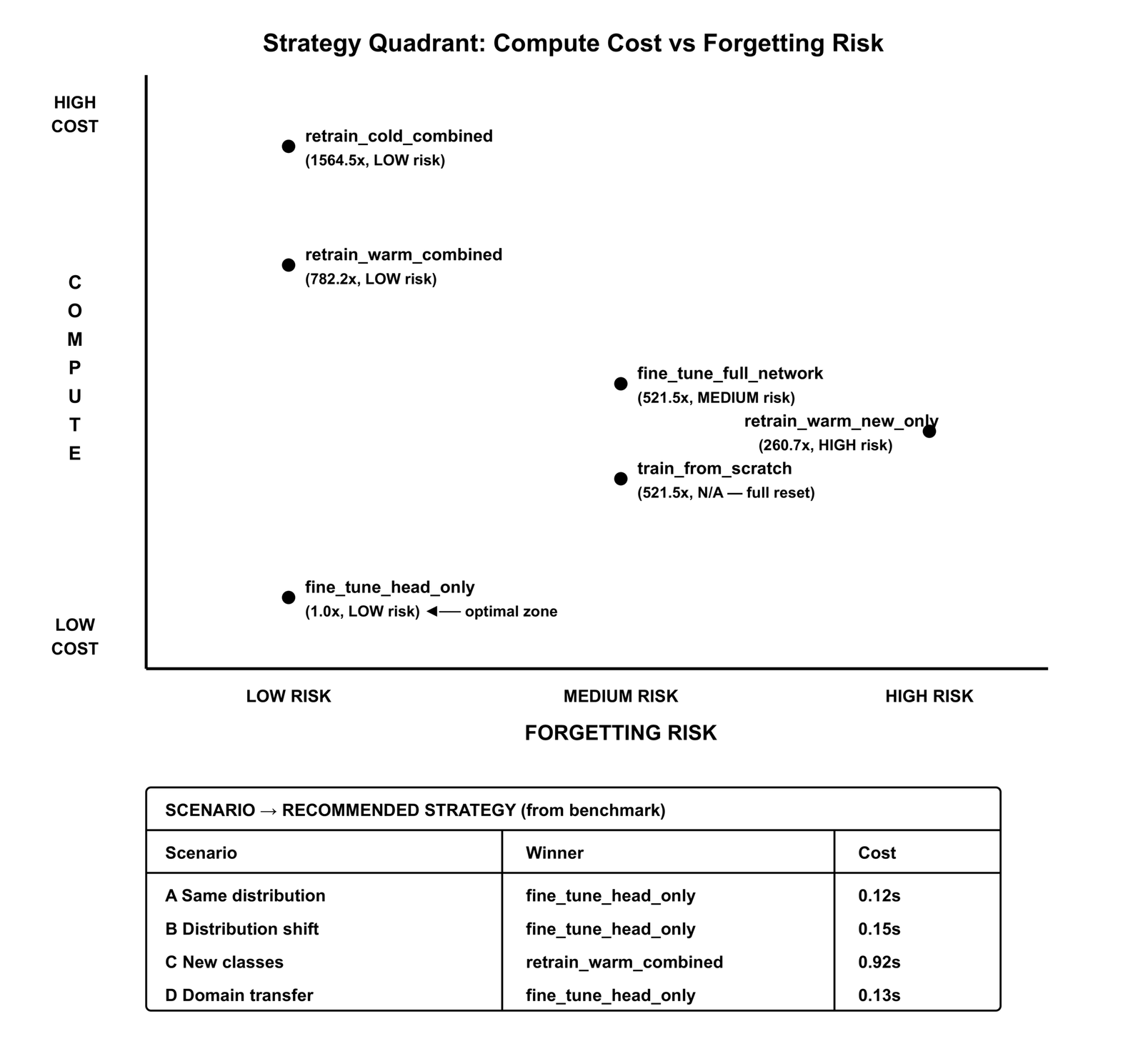
COST MODEL — Relative estimates (fine_tune_head_only = 1.0x baseline) Params total: 267,000 | Head: 512 | New samples: 500 | Historical: 1,000
| Strategy | Compute | Samples | Forgetting Risk |
|---|---|---|---|
| fine_tune_head_only | 1.0x | 500 | low |
| fine_tune_full_network | 521.5x | 500 | medium |
| retrain_warm_new_only | 260.7x | 500 | high |
| retrain_warm_combined | 782.2x | 1,500 | low |
| retrain_cold_combined | 1,564.5x | 1,500 | low |
| train_from_scratch | 521.5x | 500 | n/a (complete reset) |
Head-only fine-tuning is not marginally cheaper. It is 521x cheaper than full fine-tuning on the same dataset.
If your system retrains 50 times per year and fine-tuning is adequate for your scenario, that difference is not a rounding error. It is the difference between a retraining job that runs in seconds and one that runs in hours at scale.
The forgetting risk column is the other side of that equation. Head-only fine-tuning at 521x cheaper carries low forgetting risk because the trunk is frozen. Retrain warm new-only at 260x the baseline carries high forgetting risk because nothing prevents the gradient from overwriting prior knowledge [4]. Cost and forgetting risk are not the same axis. They have to be evaluated together.
5 Common Mistakes in ML Retraining Decisions
Mistake 1: Fine-tuning on new data only when historical data is available. If you have retained prior training data and you are fine-tuning on new data exclusively, you are accepting unnecessary forgetting risk. Retrain warm combined is almost always better if the data exists.
Mistake 2: Using a calendar schedule instead of drift-based triggers. Monthly retraining on a stable distribution wastes compute. No retraining on a drifting distribution destroys performance. Use the drift detector as the trigger, not the calendar [7].
Mistake 3: Evaluating the challenger only on new-distribution data. A model that improves on the new distribution while degrading on the old one is not an improvement. The evaluation gate must measure both.
Mistake 4: Using a high learning rate for full fine-tuning. Full fine-tuning at the same LR as initial training destroys prior representations in the first epoch. Use 10x lower [3]. This is not a minor tuning note — it is the mechanism that separates effective full fine-tuning from catastrophic forgetting disguised as retraining.
Mistake 5: Skipping the linear probe before choosing a strategy. If you do not know your trunk’s transfer quality, you cannot make an informed decision between head-only and full fine-tuning [2]. A linear probe is one training run with a frozen trunk. The result tells you directly how useful the trunk’s representations are for the new task.
Connecting to Production: Where This Fits in the Series
Articles 05, 06, and 07 each addressed a variant of the same problem — how do you keep a deployed model current as the world changes?
Article 05 prevented catastrophic forgetting during batch retraining. Article 06 adapted continuously without batches. Article 07 distinguished the three structural scenarios [6] that determine which methods are even valid.
This article adds the decision layer on top of all three. Before you implement EWC [4], before you build a replay buffer, before you deploy a streaming pipeline — you need to know whether your problem is a fine-tuning problem, a retraining problem, or a from-scratch problem. Getting that wrong makes the implementation irrelevant.
The integration with the retraining pipeline from Article 03 is direct. The drift trigger fires. The evaluation gate runs the challenger against the champion. The decision engine from this article recommends a strategy based on available signals. The registry from Article 04 handles the promotion. Those four pieces — trigger, strategy selection, training, promotion — are the complete production retraining loop.
# Evaluation gate — extends the Article 03 gate with forgetting checks
def passes_evaluation_gate(
    challenger               : CLMetrics,
    champion                 : CLMetrics,
    max_forgetting_threshold : float = 0.05,
) -> bool:
    # Gate 1: New task accuracy must improve or hold
    if challenger.acc < champion.acc - 0.02:
        return False
    # Gate 2: Maximum forgetting must stay within SLA
    if challenger.fm > max_forgetting_threshold:
        return False
    # Gate 3: Backward transfer must not substantially degrade
    if challenger.bwt < champion.bwt - 0.03:
        return False
return TrueA challenger that improves on new data while failing Gate 2 does not get promoted. That enforcement is what separates a production ML system from a notebook experiment that sometimes works.
What Is Next
This article closes Cluster 2. Articles 05–08 together form a complete continual learning stack: preventing forgetting during retraining, adapting to streaming data, matching your architecture to your scenario, and making the strategy decision correctly before implementation begins.
Article 09 — ML Model Monitoring: How to Detect Data Drift and Model Decay in Production opens Cluster 3. Where Cluster 2 asked “how do we update the model correctly,” Cluster 3 asks “how do we know when and why the model is degrading.”
Article 09 covers statistical drift tests (KS, PSI, MMD), Evidently AI integration, Grafana and Prometheus dashboards, and how to distinguish the three failure modes — data drift, concept drift, and catastrophic forgetting — that look identical from the outside but require completely different responses.
If your deployed model is already degrading and you need to diagnose before you act, go directly to Article 09 — ML Model Monitoring.
Complete Code: https://github.com/Emmimal/Retrain-vs-Fine-Tune/
References
[1] Pan, S. J., & Yang, Q. (2010). A survey on transfer learning. IEEE Transactions on Knowledge and Data Engineering, 22(10), 1345–1359. https://doi.org/10.1109/TKDE.2009.191
[2] Yosinski, J., Clune, J., Bengio, Y., & Lipson, H. (2014). How transferable are features in deep neural networks? In Advances in Neural Information Processing Systems (NeurIPS 27) (pp. 3320–3328).
https://doi.org/10.48550/arXiv.1411.1792
[3] Howard, J., & Ruder, S. (2018). Universal language model fine-tuning for text classification. Proceedings of the 56th Annual Meeting of the Association for Computational Linguistics (ACL). https://doi.org/10.18653/v1/P18-1031
[4] Kirkpatrick, J., Pascanu, R., Rabinowitz, N., Veness, J., Desjardins, G., Rusu, A. A., Milan, K., Quan, J., Ramalho, T., Grabska-Barwinska, A., Hassabis, D., Clopath, C., Kumaran, D., & Hadsell, R. (2017). Overcoming catastrophic forgetting in neural networks. Proceedings of the National Academy of Sciences, 114(13), 3521–3526. https://doi.org/10.1073/pnas.1611835114
[5] Parisi, G. I., Kemker, R., Part, J. L., Kanan, C., & Wermter, S. (2019). Continual lifelong learning with neural networks: A review. Neural Networks, 113, 54–71. https://doi.org/10.1016/j.neunet.2019.01.012
[6] van de Ven, G. M., & Tolias, A. S. (2019). Three scenarios for continual learning. arXiv preprint. https://arxiv.org/abs/1904.07734
[7] Gama, J., Žliobaitė, I., Bifet, A., Pechenizkiy, M., & Bouchachia, A. (2014). A survey on concept drift adaptation. ACM Computing Surveys, 46(4), Article 44. https://doi.org/10.1145/2523813
[8] Paszke, A., Gross, S., Massa, F., Lerer, A., Bradbury, J., Chanan, G., Killeen, T., Lin, Z., Gimelshein, N., Antiga, L., Desmaison, A., Kopf, A., Yang, E., DeVito, Z., Raison, M., Tejani, A., Chilamkurthy, S., Steiner, B., Fang, L., Bai, J., & Chintala, S. (2019). PyTorch: An imperative style, high-performance deep learning library. Advances in Neural Information Processing Systems (NeurIPS), 32. https://proceedings.neurips.cc/paper/2019/hash/bdbca288fee7f92f2bfa9f7012727740-Abstract.html
[9] Ruder, S. (2019). Neural transfer learning for natural language processing (Doctoral thesis). National University of Ireland, Galway. https://ruder.io/thesis/
Disclosure
Code authorship: All code in this article — the MLP architecture with freeze_trunk(), expand_head(), snapshot() and restore(); the TrainFromScratch, FineTuner, and Retrainer strategy classes; the DecisionEngine and CostModel; the four scenario data generators; the StrategyMetrics evaluation framework; the PretrainedRegistry; the benchmark runner; and the 37-test unit test suite — is the original work of the author. The framework builds on PyTorch [8], an open-source deep learning library under the BSD license.
Benchmark authenticity: All benchmark numbers in this article are from real runs executed by the author on CPU (Python 3.12, PyTorch 2.0+). Seed: 42. The output shown matches logged output verbatim. No numbers were adjusted or estimated. Total benchmark runtime: 13.4 seconds.
Dataset: All experiments use synthetic Gaussian mixture datasets generated programmatically in data/generators.py. No external dataset downloads are required.
No affiliate relationships: No tools, libraries, or services are mentioned for compensation. All recommendations reflect independent technical evaluation. All referenced tools are open-source under MIT or BSD licenses.
Series affiliation: This is Article 08 of the Production ML Engineering series published at EmiTechLogic. Articles 01–07 are linked throughout where referenced.
Series: Production ML Engineering — Article 08 of 15 Previous: Continual Learning in PyTorch: A Practical Guide for ML Engineers (Article 07) Next: ML Model Monitoring: How to Detect Data Drift and Model Decay in Production (Article 09)




Leave a Reply