Shadow Deployment and Canary Testing for Machine Learning Models: A Practical Guide

Shadow deployment is one of the most effective ways to validate a machine learning model before replacing it in production. Article 10 ended with a dashboard that tells you a model is drifting or decaying. It does not tell you whether the model you are about to replace it with is actually better. That is a different problem, and it is the one that sinks more deployments than drift ever does. A team retrains a model, watches offline accuracy go up, ships it, and finds out three days later that offline accuracy and production accuracy measure two different things.

Shadow deployment and canary testing are the two techniques that close that gap. Neither is complicated in principle. Both are easy to get subtly wrong in practice, in ways that don’t throw an error—they just quietly give you the wrong confidence.

This article builds both from scratch: a shadow router that runs a candidate model on every real request without ever serving its output, a canary router that serves a candidate to a controlled slice of real traffic, and the statistical layer that decides, honestly, whether a candidate is ready to take over. Every number below is from code that ran on this machine, seed 42, nothing adjusted after the fact.

Full repository: https://github.com/Emmimal/shadow-canary-router/

What Is Shadow Deployment in Machine Learning?

Shadow deployment runs a candidate model on the same input as the production model, on every real request, and throws the candidate’s output away as far as the caller is concerned. The caller only ever sees the primary model’s prediction. The candidate’s prediction gets logged next to it for offline comparison.

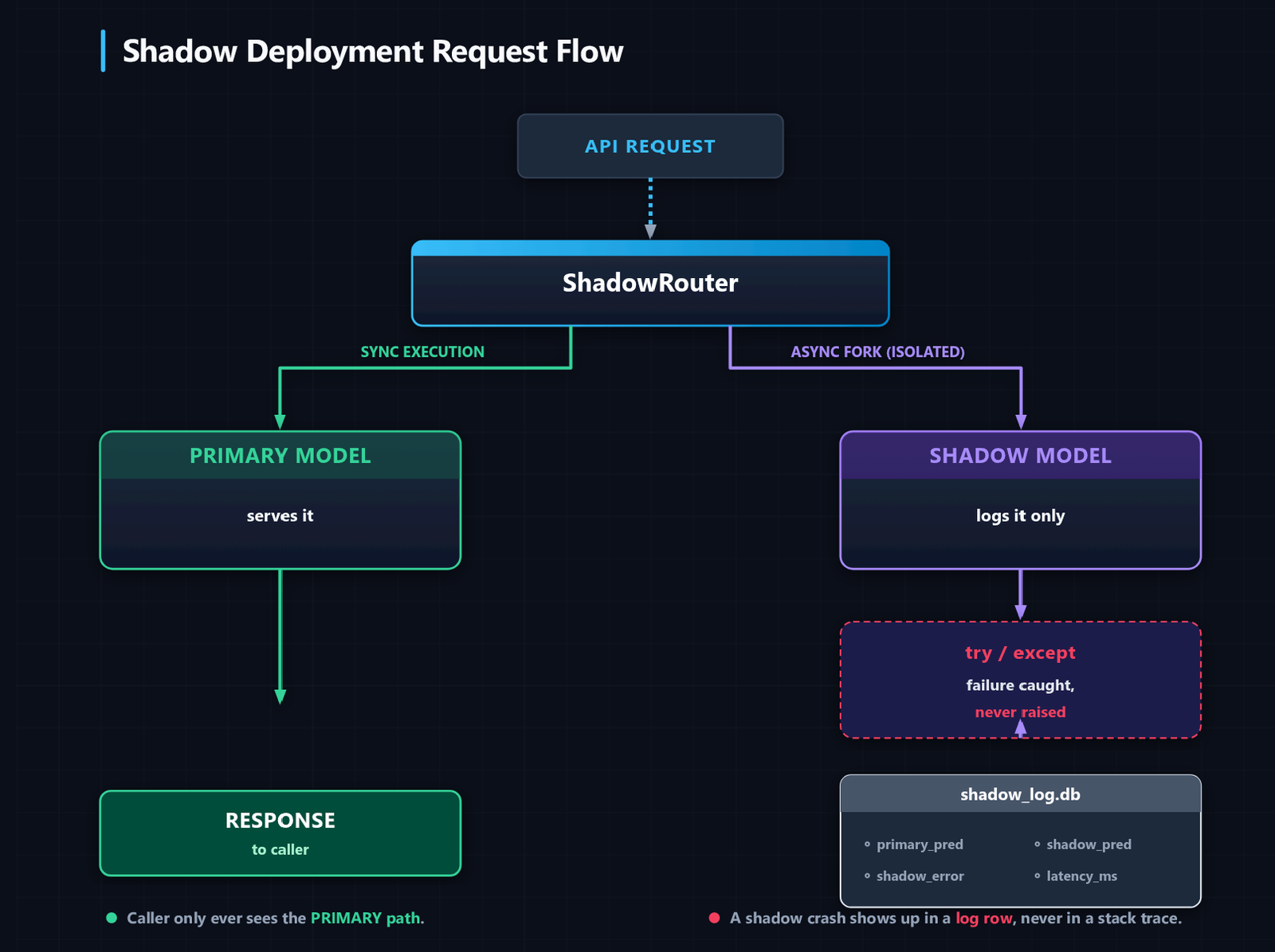
The entire value of shadow mode comes from one property: it cannot make things worse. If the candidate model is broken, crashes, returns garbage, or is slower than the primary by two orders of magnitude, none of that reaches a real user. It shows up in a log you look at later, not in someone’s application.

That property is also shadow mode’s limitation. Because the candidate’s output is never served, shadow mode cannot tell you how the candidate performs when its predictions actually drive downstream behavior, things like a recommendation a user acts on, or a fraud flag that blocks a transaction. Agreement with the primary model on paper is not the same as measured impact on outcomes. Shadow mode answers “does this model behave differently, and is that difference explainable,” not “is this model better where it counts.” Canary testing answers the second question, at the cost of exposing real traffic to real risk.

Shadow Deployment vs A/B Testing vs Canary Release

These three techniques get used interchangeably in casual conversation and that causes real confusion, because they carry genuinely different risk profiles.

Shadow deployment exposes zero real users to the candidate’s decisions. It is the only one of the three with this property, and it is why shadow mode is almost always the right first step for a model whose failure mode is expensive: fraud detection, medical triage, credit decisions. The cost is that it never validates the candidate against real-world outcomes, only against agreement with the incumbent.

Canary release exposes a small, deliberately limited slice of real traffic to the candidate. Unlike shadow mode, this is real risk: a canary user genuinely receives the candidate’s prediction. The traffic percentage is the dial that controls blast radius, and the whole discipline of canary testing is choosing that percentage, and the promotion criteria, so the blast radius stays small until you have evidence the candidate deserves more.

A/B testing also splits real traffic between two variants, but the intent is different. A canary test asks “is the new model safe and at least as good,” and typically ramps toward 100% once that’s answered. An A/B test asks “which of these two variants is better,” often holds both arms at a fixed split for the test’s full duration, and is frequently run to detect a specific, pre-registered effect (like a conversion lift) rather than to guard a rollout. In practice, the mechanics behind a canary router and an A/B test router are nearly identical, deterministic traffic splitting, per-arm metrics, a significance test. What differs is the stopping rule and the intent behind the split.

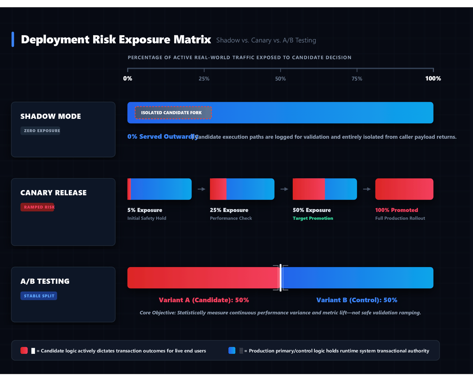
The practical sequence for a genuinely new model architecture, not a routine retrain: shadow first to catch crashes, latency problems, and gross disagreement for free. Canary second, ramping gradually, to measure real impact while bounding the damage of a candidate that looked fine in shadow but isn’t. A/B testing is a sibling technique for when the question is comparative performance between two models you’d be equally comfortable running, not a safety gate for one candidate.

How to Implement Shadow Deployment in Python (Step-by-Step)

The router is a wrapper around two predict_proba callables. It always returns the primary’s prediction. The shadow call is wrapped in its own try/except, because a shadow model raising an exception must never become a caller-visible error. That single line, a try/except around a piece of code whose result nobody consumes for the response, is the whole safety guarantee of shadow mode, and it is worth stating that plainly instead of leaving it implicit in the code.

class ShadowRouter:
    def __init__(self, primary_predict_proba, shadow_predict_proba, db_path, batch_id=0):
        self.primary_predict_proba = primary_predict_proba
        self.shadow_predict_proba = shadow_predict_proba
        self.db_path = db_path
        self.batch_id = batch_id
        init_db(db_path)

    def predict(self, request_id, features, true_class=None):
        x = features.reshape(1, -1)

        t0 = time.perf_counter()
        primary_scores = self.primary_predict_proba(x)[0]
        primary_latency_ms = (time.perf_counter() - t0) * 1000
        primary_pred = int(np.argmax(primary_scores))
        primary_conf = float(primary_scores[primary_pred])

        shadow_pred = shadow_conf = shadow_latency_ms = None
        shadow_scores = None
        shadow_error = None
        try:
            t0 = time.perf_counter()
            shadow_scores = self.shadow_predict_proba(x)[0]
            shadow_latency_ms = (time.perf_counter() - t0) * 1000
            shadow_pred = int(np.argmax(shadow_scores))
            shadow_conf = float(shadow_scores[shadow_pred])
        except Exception as e:
            # A shadow failure must never propagate to the caller.
            shadow_error = f"{type(e).__name__}: {e}"

        self._log(request_id, features, primary_pred, primary_conf, primary_scores,
                   primary_latency_ms, shadow_pred, shadow_conf, shadow_scores,
                   shadow_latency_ms, shadow_error, true_class)

        return ShadowResult(request_id, primary_pred, primary_conf, primary_latency_ms,
                             shadow_pred, shadow_conf, shadow_latency_ms, shadow_error)

class ShadowRouter:
    def __init__(self, primary_predict_proba, shadow_predict_proba, db_path, batch_id=0):
        self.primary_predict_proba = primary_predict_proba
        self.shadow_predict_proba = shadow_predict_proba
        self.db_path = db_path
        self.batch_id = batch_id
        init_db(db_path)

    def predict(self, request_id, features, true_class=None):
        x = features.reshape(1, -1)

        t0 = time.perf_counter()
        primary_scores = self.primary_predict_proba(x)[0]
        primary_latency_ms = (time.perf_counter() - t0) * 1000
        primary_pred = int(np.argmax(primary_scores))
        primary_conf = float(primary_scores[primary_pred])

        shadow_pred = shadow_conf = shadow_latency_ms = None
        shadow_scores = None
        shadow_error = None
        try:
            t0 = time.perf_counter()
            shadow_scores = self.shadow_predict_proba(x)[0]
            shadow_latency_ms = (time.perf_counter() - t0) * 1000
            shadow_pred = int(np.argmax(shadow_scores))
            shadow_conf = float(shadow_scores[shadow_pred])
        except Exception as e:
            # A shadow failure must never propagate to the caller.
            shadow_error = f"{type(e).__name__}: {e}"

        self._log(request_id, features, primary_pred, primary_conf, primary_scores,
                   primary_latency_ms, shadow_pred, shadow_conf, shadow_scores,
                   shadow_latency_ms, shadow_error, true_class)

        return ShadowResult(request_id, primary_pred, primary_conf, primary_latency_ms,
                             shadow_pred, shadow_conf, shadow_latency_ms, shadow_error)

Shadow Deployment Logging Schema

The log needs one row per request, with both models’ outputs plus enough metadata to reconstruct what happened later:

SCHEMA = """
CREATE TABLE IF NOT EXISTS shadow_log (
    id INTEGER PRIMARY KEY AUTOINCREMENT,
    request_id TEXT NOT NULL,
    batch_id INTEGER NOT NULL,
    features TEXT NOT NULL,
    primary_pred INTEGER NOT NULL,
    primary_conf REAL NOT NULL,
    primary_scores TEXT NOT NULL,
    shadow_pred INTEGER,
    shadow_conf REAL,
    shadow_scores TEXT,
    primary_latency_ms REAL NOT NULL,
    shadow_latency_ms REAL,
    shadow_error TEXT,
    true_class INTEGER,
    logged_at REAL NOT NULL
);
CREATE INDEX IF NOT EXISTS idx_shadow_batch ON shadow_log(batch_id);
"""

SCHEMA = """
CREATE TABLE IF NOT EXISTS shadow_log (
    id INTEGER PRIMARY KEY AUTOINCREMENT,
    request_id TEXT NOT NULL,
    batch_id INTEGER NOT NULL,
    features TEXT NOT NULL,
    primary_pred INTEGER NOT NULL,
    primary_conf REAL NOT NULL,
    primary_scores TEXT NOT NULL,
    shadow_pred INTEGER,
    shadow_conf REAL,
    shadow_scores TEXT,
    primary_latency_ms REAL NOT NULL,
    shadow_latency_ms REAL,
    shadow_error TEXT,
    true_class INTEGER,
    logged_at REAL NOT NULL
);
CREATE INDEX IF NOT EXISTS idx_shadow_batch ON shadow_log(batch_id);
"""

shadow_pred, shadow_conf, and shadow_error are all nullable, and exactly one of “shadow has a prediction” or “shadow has an error” is true for any row. This schema, and the numpy-scalar JSON encoder needed to serialize the score vectors, follow the same pattern established in Article 10’s monitoring store: build your monitoring dashboard covers that encoder bug in detail if you haven’t hit it yet.

Verifying the Shadow Deployment Failure Isolation Guarantee

This is the one property in this article that is worth a dedicated test, not just a benchmark, because a regression here is invisible until a shadow model actually breaks in production:

class RaisingModel:
    def predict_proba(self, X):
        raise RuntimeError("shadow model exploded")

def test_shadow_failure_does_not_raise(db_path):
    router = ShadowRouter(DummyModel(fixed_class=0).predict_proba, RaisingModel().predict_proba, db_path)
    result = router.predict("req-2", np.zeros(5), true_class=0)
    assert result.primary_pred == 0
    assert result.shadow_pred is None
    assert result.shadow_error is not None

class RaisingModel:
    def predict_proba(self, X):
        raise RuntimeError("shadow model exploded")

def test_shadow_failure_does_not_raise(db_path):
    router = ShadowRouter(DummyModel(fixed_class=0).predict_proba, RaisingModel().predict_proba, db_path)
    result = router.predict("req-2", np.zeros(5), true_class=0)
    assert result.primary_pred == 0
    assert result.shadow_pred is None
    assert result.shadow_error is not None

This test, and 22 others covering the router, the canary splitter, and the statistics layer, all pass. The full suite runs in about a second.

Measuring Shadow Deployment Performance

Running two models per request is not free, and the naive version of shadow mode, calling the shadow model synchronously inside the request handler, adds that cost directly to your response latency. I benchmarked this directly: a logistic regression primary against a 150-tree random forest candidate, five trials of 500 single-row predictions each, median reported because per-call timing at sub-millisecond scale is noisy.

That is roughly 111 times slower, and the entire difference is the shadow model’s own inference cost, not any overhead from the router itself. A heavier candidate architecture, which is common, since the whole point of testing a candidate is often that it’s a bigger, more expensive model, means synchronous shadow calls can dominate your response time. The fix is the same one Article 10 used for drift computation: don’t do it in the request path. Fire the shadow call asynchronously, log the result when it completes, and let the caller’s response go out as soon as the primary model answers. The router as written above is deliberately synchronous, for clarity and for the benchmark; a production deployment should queue the shadow call to a background worker or a fire-and-forget task instead of awaiting it inline.

Canary Testing for ML: Gradual Traffic Rollout Explained

Canary testing takes the miner’s-canary framing literally: expose a small population to the new thing, watch closely, and only expand exposure once you have evidence it’s safe. For an ML model, “exposure” means a fraction of real requests get the candidate’s prediction instead of the primary’s, and “evidence” means a statistical comparison of outcomes between the two groups, not a vibe.

Setting Traffic Split Percentages

The split has to satisfy two properties that are easy to state and easy to get wrong. First, deterministic: the same entity (user, session, account) should land in the same arm every time, for the duration of the test, or their individual experience becomes incoherent and any per-entity effect gets smeared across both arms. Second, adjustable: you need to change the percentage without redeploying, since a canary test that starts at 5% and needs a code push to reach 25% defeats the purpose of gradual rollout.

Hashing the entity ID solves both. This is the same idea behind consistent hashing in distributed caching, applied to a much simpler two-bucket case:

def assign_arm(entity_id: str, canary_pct: float, salt: str = "canary-v1") -> str:
    digest = hashlib.sha256(f"{salt}:{entity_id}".encode()).hexdigest()
    bucket = int(digest[:8], 16) / 0xFFFFFFFF
    return "canary" if bucket < canary_pct else "control"

def assign_arm(entity_id: str, canary_pct: float, salt: str = "canary-v1") -> str:
    digest = hashlib.sha256(f"{salt}:{entity_id}".encode()).hexdigest()
    bucket = int(digest[:8], 16) / 0xFFFFFFFF
    return "canary" if bucket < canary_pct else "control"

salt exists so you can re-randomize every entity’s assignment when starting a fresh test, without which a user who happened to land in the canary arm on one test would systematically land there again on the next, correlating results across unrelated tests.

I verified the split actually produces the requested ratio, and that it’s stable per entity, across 20,000 synthetic users at four percentages:

The small deviation from the requested percentage (5.12% instead of exactly 5.00%) is sampling noise from a finite population hashing into a continuous bucket range, not a bug in the hash. It shrinks as the entity population grows.

Statistical Validation for Shadow Deployment

Shadow and canary comparisons need two different statistical tests, because they’re asking two different questions on two different data structures.

Shadow vs primary is a paired comparison: both models see the identical input, so the right question is “do they agree, and when they disagree, which one is actually right.” Agreement rate alone is a first pass. The sharper tool is McNemar’s test, run only on the discordant pairs, the cases where the two models disagree. It’s a standard tool for comparing paired classifier predictions for exactly this reason, and it exists specifically because a plain proportion test assumes independent samples, which paired predictions on the same inputs are not.

b, c = primary_only_correct, shadow_only_correct
if b + c < 25:
    p_value = 2 * stats.binom.cdf(min(b, c), b + c, 0.5)
else:
    mcnemar_stat = (abs(b - c) - 1) ** 2 / (b + c)
    p_value = 1 - stats.chi2.cdf(mcnemar_stat, df=1)

b, c = primary_only_correct, shadow_only_correct
if b + c < 25:
    p_value = 2 * stats.binom.cdf(min(b, c), b + c, 0.5)
else:
    mcnemar_stat = (abs(b - c) - 1) ** 2 / (b + c)
    p_value = 1 - stats.chi2.cdf(mcnemar_stat, df=1)

The < 25 branch uses an exact binomial test instead of the chi-square approximation, since the continuity-corrected chi-square form gets unreliable with very few discordant pairs.

I ran this on two candidates against the same primary, 1,500 requests each. The first candidate is a genuinely stronger model (a random forest against the primary’s logistic regression). The second has a realistic, silent defect: its feature columns are served in the wrong order, a column-mismatch bug that never raises an error because the shapes still match.

Both rows show a highly significant McNemar result, and that’s the point: the test tells you the disagreement is not noise, but it does not tell you which direction is good. You have to read the counts. In the first row, the shadow model is correct 256 times where the primary is wrong, against only 25 times the reverse, a lopsided win. In the second row, the primary is correct 649 times where the shadow model is wrong, against only 140 times the reverse, a lopsided loss. The offline accuracy numbers confirm it: 87.2% for the genuinely better candidate, 38.5% for the column-mismatch one, against a 71.6% primary. Shadow mode caught the second candidate’s defect using zero production incidents, entirely from agreement statistics on live traffic it never got to influence.

Canary vs control is the opposite structure: independent samples, since canary and control serve disjoint sets of real requests, and the outcome that matters is measured accuracy once ground truth lands, not agreement. A two-proportion z-test is the right tool here:

p_pool = (control_correct.sum() + canary_correct.sum()) / (n_c + n_t)
se = np.sqrt(p_pool * (1 - p_pool) * (1 / n_c + 1 / n_t))
z = (acc_t - acc_c) / se
p_value = 2 * (1 - stats.norm.cdf(abs(z)))

p_pool = (control_correct.sum() + canary_correct.sum()) / (n_c + n_t)
se = np.sqrt(p_pool * (1 - p_pool) * (1 / n_c + 1 / n_t))
z = (acc_t - acc_c) / se
p_value = 2 * (1 - stats.norm.cdf(abs(z)))

When to Promote a Shadow Deployment Candidate

A promotion decision needs a hard gate on sample size that runs before the p-value gets looked at, not after. The reason is subtle: the normal approximation behind a two-proportion z-test gets shaky with only a handful of observations in either arm, and a “significant” result on 40 requests is not the same claim as a significant result on 2,000, even when the arithmetic produces the same p-value. I set the gate at 200 samples per arm and treat anything below that as automatically inconclusive, regardless of what the p-value says:

if not min_sample_met:
    recommendation = "hold_insufficient_sample"
elif significant and delta > min_practical_delta:
    recommendation = "promote"
elif significant and delta < -min_practical_delta:
    recommendation = "rollback"
else:
    recommendation = "hold_no_significant_difference"

if not min_sample_met:
    recommendation = "hold_insufficient_sample"
elif significant and delta > min_practical_delta:
    recommendation = "promote"
elif significant and delta < -min_practical_delta:
    recommendation = "rollback"
else:
    recommendation = "hold_no_significant_difference"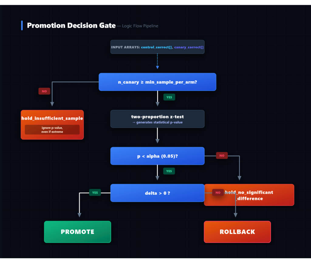

I ran the genuinely-better candidate through a three-stage ramp, 5% then 25% then 50% of traffic, 800 requests per stage:

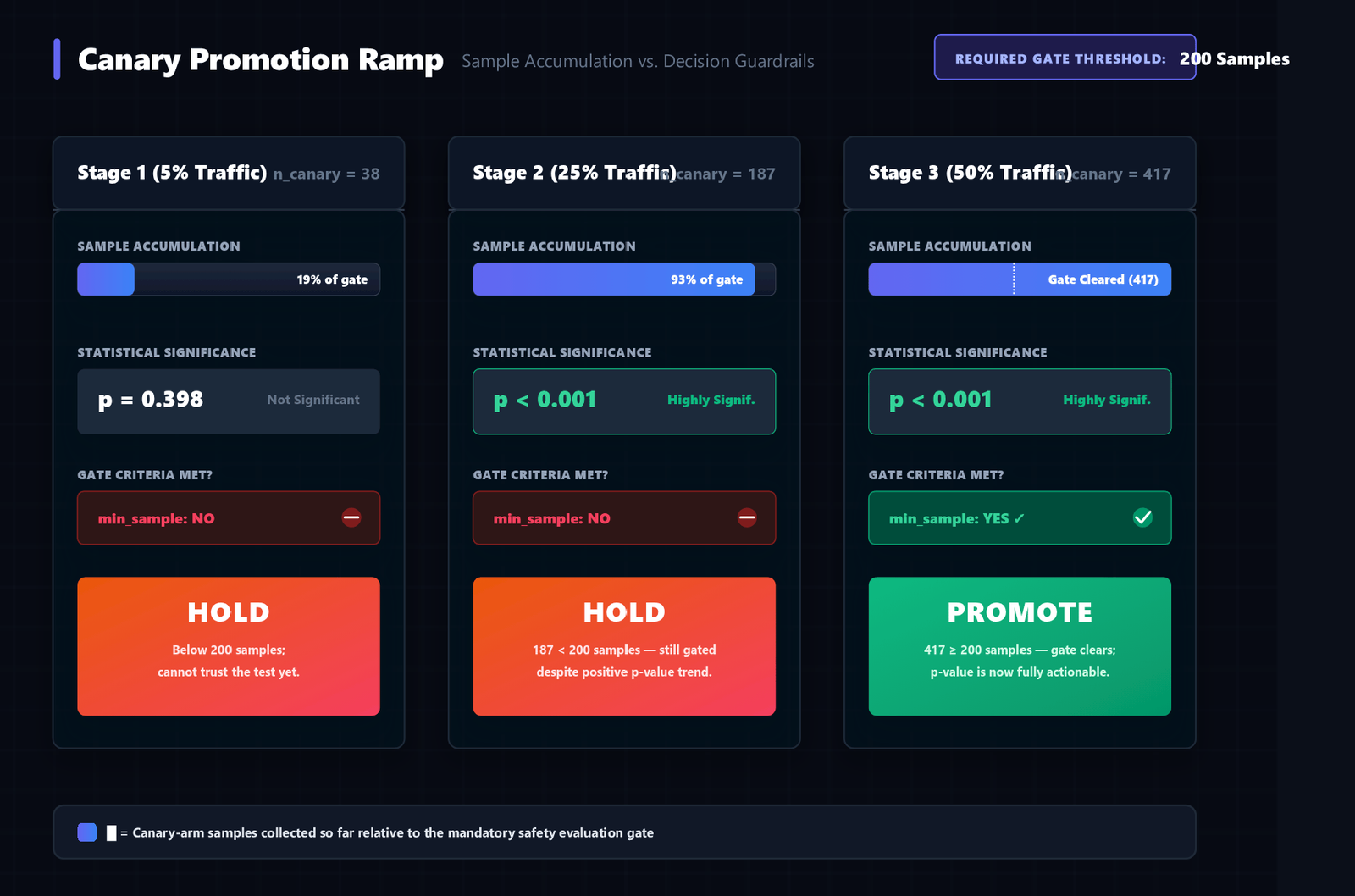
Stage 2 is the interesting row. The p-value is already far below any reasonable threshold, and the accuracy gap is large and in the obviously right direction. The system still holds, because the canary arm has 187 samples against a 200 minimum. That’s a real cost: a genuinely better model waits one more stage before the router will recommend promoting it. It’s a cost I chose deliberately, because the alternative, letting an extreme but small-sample p-value trigger promotion, is exactly the failure mode that makes a promotion gate untrustworthy.

The buggy candidate makes the opposite case for the same gate. I ran it at a fixed 10% canary split and checked the decision at five points as traffic accumulated:

At 400 total requests, the p-value already reflects a real, severe defect, a 36-point accuracy gap. The gate still holds, because only 44 canary samples exist at a 10% split. It takes 2,500 total requests, 242 of them landing in the canary arm, before the system will actually recommend rollback. That delay is the direct, quantifiable cost of running a cautious initial canary percentage: the lower the percentage, the longer it takes to accumulate enough canary-arm samples to clear the gate, no matter how obvious the defect is in the data you already have. This is the actual argument for starting a canary at a higher percentage when the downside of a bad candidate is bounded, and for starting lower only when it genuinely isn’t.

Tools: Seldon Core, BentoML, and AWS SageMaker for Shadow Deployment

These three sit at different points between “you write the routing logic” and “the platform writes it for you.”

Seldon Core runs on Kubernetes and treats shadow and canary as first-class deployment primitives in its inference graph configuration: you declare a shadow deployment alongside a primary model, and the platform handles duplicating traffic to it. This buys you infrastructure-level correctness, no request ever reaches the shadow model through code you wrote, at the cost of committing to Kubernetes and Seldon’s CRDs as your serving layer.

BentoML is closer to the code-first approach in this article. It packages models as services with a clean Python API and leaves routing logic, including anything shadow- or canary-shaped, to whatever framework sits in front of it. That gives you the same flexibility this article’s router has, with BentoML handling packaging, versioning, and serving instead of you writing that layer yourself.

AWS SageMaker supports both patterns as managed inference features: shadow variants on a SageMaker endpoint mirror traffic to a shadow model and log comparison metrics without code, and production variants let you split traffic by weight across model versions on the same endpoint, which is SageMaker’s version of a canary. The tradeoff is the same one that shows up whenever a managed platform absorbs a pattern like this: less code to maintain, less visibility into exactly how the comparison logic works, and a harder time reproducing the same statistics outside AWS’s dashboards if you need to.

The practical recommendation: if you’re already committed to Kubernetes, Seldon’s native primitives are worth using over building your own. If you’re on SageMaker for serving already, its built-in shadow variants and weighted routing cover most of what this article built, with less code. If you want the statistics themselves, agreement rate, McNemar’s test, the promotion gate, to be something you can inspect, modify, and reuse across projects that don’t share a serving platform, the from-scratch version in this article is the one that travels with you.

Shadow Deployment FAQ

Key Takeaways

Shadow deployment’s entire value is that it cannot make things worse. The moment a shadow call becomes synchronous and blocking in the request path, you’ve traded away exactly the property that made it safe to run in the first place, one this benchmark shows adding roughly 111x to per-request latency with a heavier candidate model.

Agreement rate is a first pass, not the test. McNemar’s test on the discordant pairs is the right tool for paired shadow-vs-primary comparisons, and it will hand you a highly significant result in both directions, when a candidate is genuinely better and when it’s silently broken. The p-value tells you the disagreement is real; you still have to read which side is actually correct.

A promotion or rollback decision needs a sample-size gate that runs before the p-value, not after. This benchmark’s buggy-candidate progression shows a p-value under 0.001 sitting there for over 2,000 requests while the gate correctly holds, because the canary arm hadn’t yet crossed 200 samples. That’s not the statistics failing; that’s the gate doing exactly what it’s supposed to do.

Canary percentage is a dial with a real, measurable cost on both ends. Too low, and a genuinely broken candidate takes far longer to accumulate enough canary-arm samples to trigger a rollback. Too high, and you’ve widened the blast radius of a candidate you haven’t validated yet. Neither extreme is free.

Deterministic, hash-based traffic splitting is what makes a canary percentage adjustable without a redeploy and keeps any individual entity’s experience coherent for the duration of a test. A random per-request coin flip does neither.

What Is Next

Article 12 turns to a different kind of production symptom: an inference service that’s technically up but has gotten slow, and the process of finding out why. The same synchronous-shadow-call latency benchmark in this article is a small preview of that problem, one blocking call added roughly 8.5 milliseconds to every request in a test where it should have added close to zero. Article 12 covers profiling a live model to find where time is actually going, and the tradeoffs between batching, quantization, and hardware choices once you know.

If the candidate that clears your canary gate came out of an automated retraining pipeline, the promotion decision in this article is the natural gate to put between that pipeline and a full deployment: retrain, shadow, canary, promote, in that order, with a model registry recording which version is serving at each stage. See the Production ML Engineering guide for how all of these pieces connect end to end.

References

[1] McNemar, Q. (1947). Note on the sampling error of the difference between correlated proportions or percentages. Psychometrika, 12(2), 153-157. https://doi.org/10.1007/BF02295996

[2] Raschka, S. (2018). Model evaluation, model selection, and algorithm selection in machine learning. arXiv preprint. Section 4.3 covers McNemar’s test for comparing classifiers. https://arxiv.org/abs/1811.12808

[3] Karger, D., Lehman, E., Leighton, T., Panigrahy, R., Levine, M., & Lewin, D. (1997). Consistent hashing and random trees: Distributed caching protocols for relieving hot spots on the World Wide Web. Proceedings of the 29th ACM Symposium on Theory of Computing (STOC), 654-663. https://doi.org/10.1145/258533.258660

[4] Google SRE Workbook. (2018). Canarying releases. https://sre.google/workbook/canarying-releases/

[5] Kreuzberger, M., Schmid, K., & Breitenöder, T. A. B. (2020). Challenges and best practices for MLOps and continuous delivery for machine learning. 2020 IEEE International Conference on Software Architecture Companion (ICSA-C). https://ieeexplore.ieee.org/document/10081336

[6] Pedregosa, F., Varoquaux, G., Gramfort, A., Michel, V., Thirion, B., Grisel, O., et al. (2011). Scikit-learn: Machine learning in Python. Journal of Machine Learning Research, 12, 2825-2830. http://jmlr.org/papers/v12/pedregosa11a.html

Disclosure

Code authorship: All code in this article, the shadow router with its failure-isolation guarantee, the deterministic hash-based canary splitter, the McNemar comparison and two-proportion promotion gate, the two-candidate benchmark pipeline, and the 23-test unit suite, is the original work of the author. The synthetic classification data and model training use scikit-learn’s make_classification, LogisticRegression, and RandomForestClassifier directly. The framework builds on NumPy, SciPy, and scikit-learn, all open-source under BSD licenses.

Benchmark authenticity: All numbers in this article, the shadow agreement statistics for both candidates, the traffic-split verification across four percentages, the three-stage canary ramp, the five-checkpoint buggy-candidate progression, and the five-trial latency comparison, are from real runs executed by the author on CPU (Python 3.12.3, NumPy 2.4, SciPy 1.17, scikit-learn 1.8). Seed: 42 throughout. Total runtime across the test suite and all benchmark scripts: approximately 67 seconds. No numbers were adjusted or estimated.

No affiliate relationships: No tools, libraries, or services are mentioned for compensation. All comparisons reflect independent technical evaluation.

Series affiliation: This is Article 11 of the Production ML Engineering series. Article 10: ML Monitoring Dashboard covers the detectors this article’s promotion decisions would ultimately feed. See also deploying a model to production, building a retraining pipeline, and model versioning.