

How to Debug ML Inference Latency and Throughput Issues
ML inference latency issues are rarely caused by the model itself. Most “why is my model slow” investigations start with guesswork instead of measurement.
Article 11 ended with a synchronous shadow call adding roughly 111x to per-request latency. One blocking call, and a fast endpoint turned slow. That number was really a preview of a bigger problem. Most “why is my model slow” investigations don’t start with a profiler. They start with someone wrapping time.time() around whatever chunk of code they suspect and hoping.
TL;DR
- Full diagnostic workflow below, real numbers, nothing estimated.
- The forward pass is rarely the bottleneck. Preprocessing and batching usually cost more.
- Quantization gave me three different answers across three identical runs. ONNX Runtime didn’t.
- Pruning never made this model faster. Once it made it slower.
- The scaling benchmark measured my laptop as much as it measured my code.
Everything here runs against one mid-sized PyTorch classifier, 528,138 parameters, four linear layers, so every technique gets tested on the same model. Windows, 4 cores, Python 3.12.10, PyTorch 2.13.0. Seed 42. Nothing adjusted after the fact, including the two sections where the numbers disagreed between runs. I kept those in, because the disagreement turned out to be the actual lesson, not something to average away before publishing.
Complete code, all scripts and the test suite: https://github.com/Emmimal/inference-latency-debugger
Why ML Inference Latency Rarely Comes From the Model
I’ve never once had “the model is slow” turn out to mean the model was slow. A forward pass has four stages: preprocessing, data movement, the model call itself, postprocessing. The model call is usually the least likely of the four to be where the time actually went. I build a naive and a fixed version of each stage, time both, and only then bring in a profiler for the forward pass itself.
Order matters here. Profile the forward pass before you’ve ruled out preprocessing and you’ll optimize something that was never the problem.
I ran every benchmark below at least twice. Two of them, quantization and scaling, came back inconsistent. I’m reporting every run for those, not the cleanest one.
Common Causes of ML Inference Latency (And How to Diagnose Each)
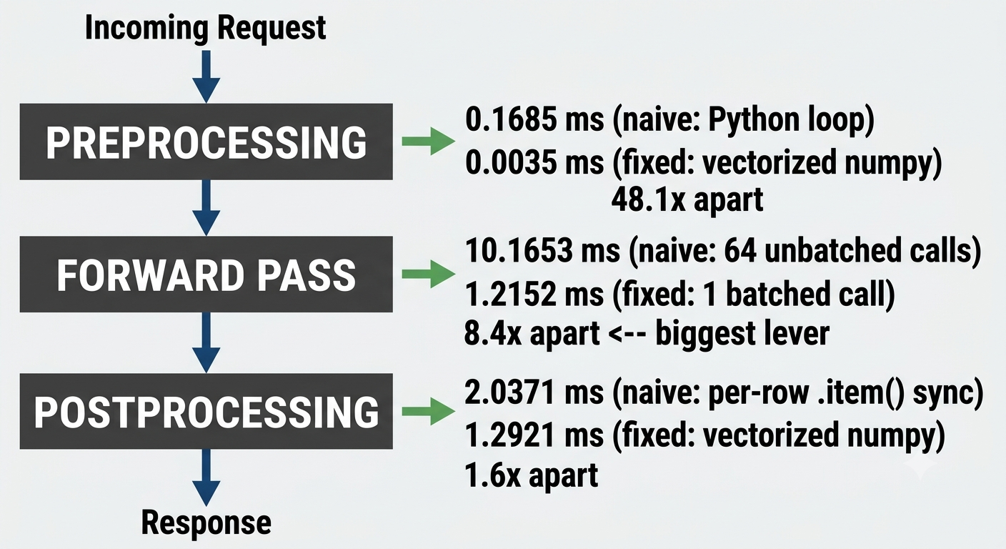
Four things hide latency, in my experience: feature scaling written as a Python loop instead of a vectorized numpy op, the model called once per row instead of once per batch, and predictions pulled off the output tensor one at a time with .item() instead of read as an array. I built naive and fixed versions of each. Full code in diagnose_causes.py.
Warmup, then 200-500 timed calls, same 4-core Windows machine:
| Cause | Naive | Fixed | Slowdown |
|---|---|---|---|
| Per-feature scaling in a Python loop (1 row) | 0.1685 ms | 0.0035 ms | 48.1x |
| Per-row model calls instead of one batched call (64 rows) | 10.1653 ms | 1.2152 ms | 8.4x |
Per-row .item() sync in postprocessing (64 rows) | 2.0371 ms | 1.2921 ms | 1.6x |
Unbatched inference is the biggest lever here, and it’s not close. Every model() call pays fixed dispatch overhead: kernel launch, autograd bookkeeping, the Python-to-C++ crossing. Call it once with 64 rows and you pay that overhead once instead of 64 times. The Python loop shows the highest ratio, 48.1x, but it’s cheap in absolute terms, about 0.17ms, which is exactly how it hides from a coarse “time the whole request” measurement. You don’t feel it until you isolate it.
How to Profile ML Inference Latency with PyTorch
Once the forward pass itself looks slow, torch.profiler tells you which operator inside it is spending the time. A profile() context around a warmed-up forward pass, record_function markers around the forward and postprocessing steps. Full script in profiler_demo.py.
Real output, 50 iterations, batch size 64:
| Name | Self CPU % | Self CPU | CPU Total % | CPU Total | CPU Time Avg | # of Calls |
|---|---|---|---|---|---|---|
| full_inference_step | 5.44% | 4.374 ms | 100.00% | 80.424 ms | 80.424 ms | 1 |
| forward_pass | 8.87% | 7.136 ms | 89.33% | 71.839 ms | 1.437 ms | 50 |
| aten::linear | 2.24% | 1.805 ms | 76.73% | 61.707 ms | 308.533 µs | 200 |
| aten::addmm | 64.34% | 51.742 ms | 67.30% | 54.123 ms | 270.616 µs | 200 |
| aten::t | 2.86% | 2.303 ms | 7.18% | 5.778 ms | 28.891 µs | 200 |
| aten::transpose | 3.93% | 3.162 ms | 4.32% | 3.475 ms | 17.375 µs | 200 |
| aten::relu | 1.63% | 1.308 ms | 3.73% | 2.996 ms | 19.977 µs | 150 |
| aten::clamp_min | 2.10% | 1.689 ms | 2.10% | 1.689 ms | 11.257 µs | 150 |
| aten::copy_ | 1.89% | 1.518 ms | 1.89% | 1.518 ms | 7.589 µs | 200 |
| aten::expand | 0.74% | 597.600 µs | 0.99% | 795.600 µs | 3.978 µs | 200 |
| aten::as_strided | 0.64% | 511.200 µs | 0.64% | 511.200 µs | 1.278 µs | 400 |
aten::addmm, the matmul inside every nn.Linear, is 64.34% of self CPU time on its own. 67.30% counting everything it calls. 200 calls, 50 iterations across 4 linear layers, about 270 microseconds each. relu and clamp_min together don’t crack 6%. I got roughly this same shape, addmm dominating in the high 60s to low 70s percent, on a completely different machine (single-core Linux) while building this article. For a dense feedforward net, the matmul is going to be the bottleneck almost everywhere. That’s where the fix needs to point.
Read Self CPU % for time spent inside the operator itself. CPU total % adds in everything it calls. Close together, like addmm here, means the operator is doing real work, not handing off to something else.
Batching Strategies to Reduce ML Inference Latency
Swept batch size 1 through 256. Throughput is batch_size / mean_latency_seconds. Full sweep in batch_vs_realtime.py.
| Batch size | Mean latency | P95 latency | Throughput (rows/sec) |
|---|---|---|---|
| 1 | 0.1818 ms | 0.3275 ms | 5,501 |
| 2 | 0.2903 ms | 0.5147 ms | 6,890 |
| 4 | 0.2828 ms | 0.4628 ms | 14,142 |
| 8 | 0.3643 ms | 0.5721 ms | 21,959 |
| 16 | 0.4714 ms | 0.7528 ms | 33,940 |
| 32 | 0.6923 ms | 0.9470 ms | 46,223 |
| 64 | 1.2097 ms | 1.6684 ms | 52,906 |
| 128 | 1.9731 ms | 2.2786 ms | 64,871 |
| 256 | 3.9727 ms | 4.5695 ms | 64,440 |
Batch 2’s mean sits a hair above batch 4’s, which shouldn’t happen. This ran on a laptop with PyCharm and background processes fighting for the same cores, not an isolated box, so I’m calling it noise rather than pretending the curve is perfectly smooth.
More interesting: throughput dips slightly from 128 to 256 instead of climbing. Batch 1 to batch 128 multiplies the input 128x, latency only grows about 11x, the fixed dispatch overhead amortizing across more rows. Past 128, that amortization runs out of room and something else, cache behavior at this hidden-layer width would be my guess, starts pushing back. Bigger batches aren’t free forever. You have to sweep past where you assume it’ll help and check.
A real-time endpoint, fraud scoring on a single transaction, wants small batches because it can’t wait to accumulate rows, and pays for that in throughput. A batch-scoring job, nightly re-scoring a customer table, wants large batches and gets meaningfully more throughput per core for it, up to the ceiling this sweep just showed. Triton and TorchServe split the difference with dynamic batching, a short buffering window with a timeout. That’s a serving-layer decision, out of scope for what I’m benchmarking here.
ML Inference Latency Optimization: Quantization, Pruning, and ONNX
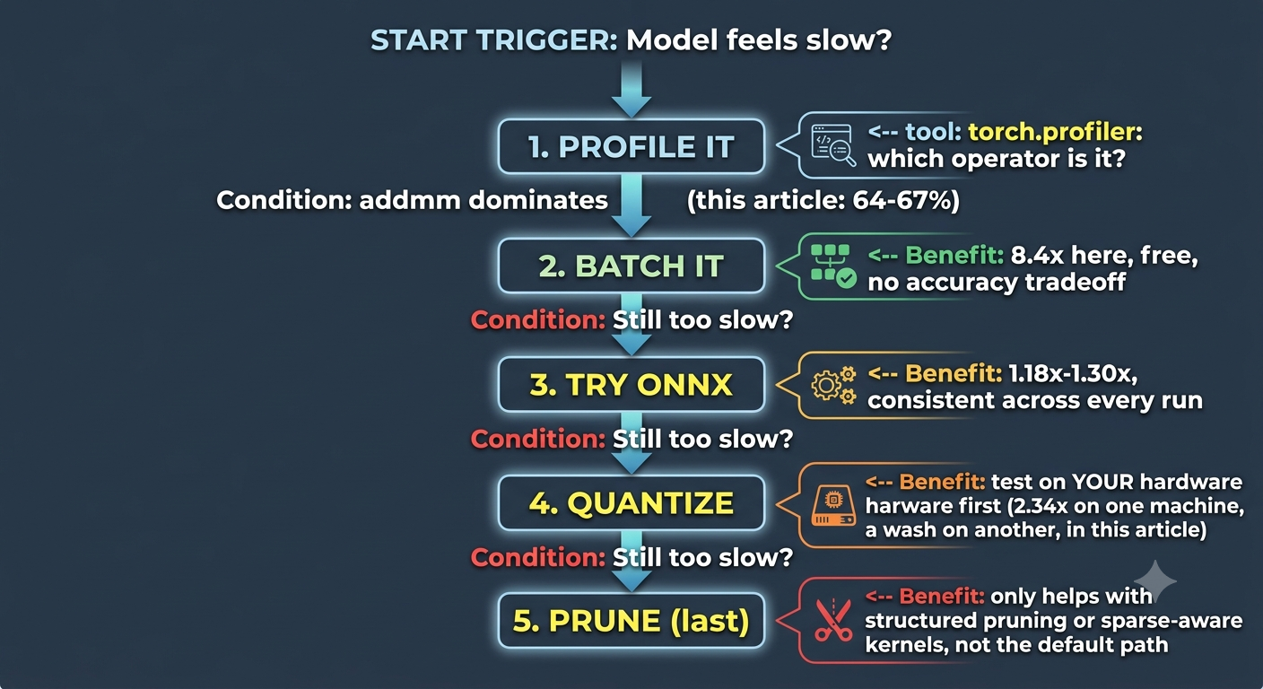
Three standard levers once the profiler points at the matmul: less precision, fewer parameters, or a different runtime. I tried all three. Only one behaved the same way twice.
Quantization in PyTorch: INT8 Step-by-Step
Dynamic quantization converts Linear weights from float32 to int8 at load time, requantizes activations on the fly, needs no calibration data, CPU only. The whole conversion:
model_int8 = torch.quantization.quantize_dynamic(model_fp32, {torch.nn.Linear}, dtype=torch.qint8)Ran it three times, back to back, same code, same machine, batch 64:
| Run | fp32 mean | int8 mean | fp32 p50 | int8 p50 |
|---|---|---|---|---|
| 1 | 1.0831 ms | 1.2801 ms | 1.0469 ms | 1.0931 ms |
| 2 | 1.0878 ms | 1.1801 ms | 1.0087 ms | 1.0840 ms |
| 3 | 1.5157 ms | 1.1706 ms | 1.1612 ms | 1.1283 ms |
Three runs, three headlines: int8 18% slower, then 8% slower, then 29% faster. Same code. If I’d run this once, whatever I got would have become the number in this article, and depending on the run, I’d have written either “don’t bother with quantization” or “free 1.3x speedup,” both wrong.
Look at run 3’s fp32 row. Mean of 1.5157ms against a p50 of 1.1612ms. P95 at 3.0126ms, p99 at 3.1796ms. That’s a fat tail. A few slow outlier calls, something else on the machine grabbing a core mid-run, dragged the mean up without touching the typical case. Int8’s row that same run has no tail like it. That asymmetry is what flipped the sign, not the technique.
P50 across all three runs tells a calmer story: int8 somewhere between 2.8% faster and 7.5% slower. Close enough to zero to call a wash on this hardware.
Size and accuracy held steady regardless. State dict went from 2066.6 KB to 525.7 KB every time, a 3.93x reduction. Predictions agreed 98.30% of the time across 2,000 fresh rows, max logit difference 0.0049, mean 0.0009. So the size and accuracy story is solid. The latency story depends on whether your CPU has a fast int8 path and whether that edge is bigger than ordinary noise. On a single-core sandbox I tested earlier, int8 won outright, 2.34x. On this 4-core Windows box, it’s a coin flip.
One environment note: PyTorch 2.13 flags torch.quantization.quantize_dynamic as deprecated, pointing at torchao as the eventual replacement. Still works, still gives the same accuracy and size numbers above. Worth checking whether torchao has stabilized before you build a new project on the old path.
If you’re deciding whether to ship quantization off a latency benchmark, run it more than once, and check p50 before you check mean.
Why Pruning Didn’t Help (And When It Would)
Next lever: zero out the smallest-magnitude weights, skip the resulting sparse compute. Global unstructured L1 pruning, 40% sparsity, every linear layer. torch.nn.utils.prune.global_unstructured with L1Unstructured. Full setup in pruning_demo.py.
| Run | Dense mean | Pruned mean | Speedup |
|---|---|---|---|
| 1 | 1.0905 ms | 1.1017 ms | 0.99x |
| 2 | 1.2786 ms | 1.4992 ms | 0.85x |
| 3 | 1.1480 ms | 1.1391 ms | 1.01x |
Verified 40.0% sparsity every run. No ambiguity to resolve with p50 here, unlike quantization, the direction is consistent: never faster, once 15% slower. torch.nn.utils.prune zeros weights but leaves the tensor dense. The addmm kernel from the profiler table still multiplies through every zero, because nothing tells it 40% of the values don’t need multiplying. It has no sparse format to exploit.
Unstructured pruning shrinks the file on disk. Useful if you’re exporting to a runtime with real sparse kernels later. It does nothing for dense CPU latency on its own, and here it occasionally cost a little. Structured pruning, removing whole neurons so the matrix is actually smaller, is the version that would show up in a latency number. Different technique, more work, not what’s tested here.
Converting to ONNX for Cross-Framework Speedup
ONNX Runtime changes the execution engine, not the weights, which is why it’s independent of quantization and, on this hardware, a lot more trustworthy. Export with torch.onnx.export(model, dummy_input, "model.onnx", dynamic_axes=..., opset_version=17, dynamo=False), load with onnxruntime.InferenceSession. Full script in onnx_demo.py.
That dynamo=False isn’t optional decoration. PyTorch 2.13 defaults to a newer torch.export-based exporter that needs onnxscript, which isn’t installed by default. Without it you get ModuleNotFoundError: No module named 'onnxscript' before export even starts. dynamo=False falls back to the older TorchScript exporter. No extra dependency, still supported, just labeled legacy.
Three runs:
| Run | Speedup (mean) | Max abs diff vs torch |
|---|---|---|
| 1 | 1.18x | 0.000000 |
| 2 | 1.30x | 0.000000 |
| 3 | 1.25x | 0.000000 |
Faster every time, in a tighter band than quantization managed even in direction, and identical output every time, max difference of exactly zero. ONNX Runtime isn’t changing the computation, only how efficiently it executes it: operator fusion, constant folding, dead node elimination, all applied at load time, none of which torch’s eager mode bothers with since it re-traces the graph shape on every call. Exported file size: 2,113,662 bytes, about 2.02MB, every run.
Set next to quantization’s coin flip, ONNX is the technique that earned its reputation here rather than only getting lucky once. If I could only try one optimization on a model like this, I’d reach for ONNX first and measure quantization on top of it after, rather than assume they stack. I haven’t tested that combination. Treat it as a guess, not a result.
Scaling ML Systems to Handle ML Inference Latency
Everything above speeds up one call. Scaling is a different question: how many requests per second can you serve past what one process handles. Worker pool behind a load balancer, one model per worker. The first version of this benchmark had a real bug, and the fix, and what happened after the fix, is the actual lesson.
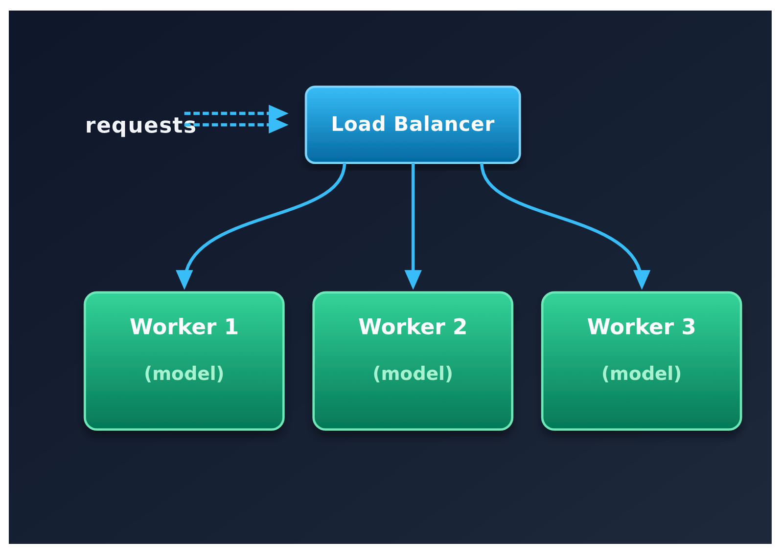
Original version spawned a fresh multiprocessing.Pool inside every call, so every worker re-imported torch from scratch before touching any real work. Windows spawns fresh interpreter processes instead of forking, unlike Linux, so that cost gets paid in full, per worker, per call. Throughput dropped as workers went up: 1,051 down to 285 requests per second across 1 to 8 workers, in one early run. Looked like scaling had failed outright.
It hadn’t. It was measuring process startup, not inference. Fix: load the model once per worker in a pool initializer, warm up before starting the timer. Full before-and-after in scaling_demo.py. That change:
| Workers | Throughput |
|---|---|
| 1 | 5,762 req/sec |
| 2 | 6,219 req/sec |
| 4 | 5,720 req/sec |
| 8 | 4,847 req/sec |
5 to 8x jump at every worker count, just from removing spawn overhead. Diagnosis confirmed. But real scaling still isn’t there. Four physical cores, and 4 workers is roughly tied with 1. Eight is worse than 1.
This machine is a laptop I do everything else on. PyCharm, background Windows processes, whatever tab is open, all pulling on the same 4 cores while this ran. The worker processes were competing with the OS for cycles instead of getting dedicated capacity to scale into. Not a flaw in the pool code. Not evidence horizontal scaling doesn’t work. A scaling benchmark measures the whole machine, and running one on shared hardware will understate your real ceiling. On dedicated infrastructure I’d expect 4 workers closer to 4x a single worker before flattening near the core count, roughly what Amdahl’s argument predicts once the parallel part actually gets dedicated cores [4].
Load balancing strategy doesn’t depend on core count, for what it’s worth. Round robin is fine when requests cost about the same. Least connections helps when they don’t, routing to whichever worker has the shortest queue instead of blind rotation. Consistent hashing, same mechanism the canary router in Article 11 used for deterministic splits [7], matters if a given user needs to land on the same worker for caching. And the autoscaling trigger should be queue depth or p95 latency, not CPU percent. CPU can sit under 50% while p95 blows past your SLA because requests batch unevenly, and CPU-based autoscaling won’t see that until it’s a problem.
Before trusting any scaling number, ask what else was running on that hardware. “It didn’t scale” and “it didn’t scale because something else was using the cores” are different findings.
Benchmarking Inference Latency: Tools and Methodology
Every number above came from the same harness in bench_utils.py. Warm up first, 20+ calls, discard them. Time 200-500 calls. Report percentiles, not a mean.
Warmup exists because the first few calls to any PyTorch model pay one-time costs, allocator warmup, lazy init, that have nothing to do with steady state and will inflate the number if you count them. Percentiles exist because a mean hides the thing you actually care about, and the quantization section above is the clearest proof of that I’ve run into personally: three identical runs, three different mean-based verdicts, one consistent verdict once p50 replaced mean. A mean from a single run told me less than a single p50 did. That gap only shows up if you run the benchmark more than once and compare both.
For load testing a live endpoint instead of a Python function, same principle, different tools depending on what you need. wrk and ab for raw HTTP load, fast, simple request-per-second numbers. Locust when the load pattern isn’t a flat blast, ramping traffic, mixed request types, think-time between calls, it’s Python-scriptable. k6 sits closer to CI, built to gate a deployment pipeline. Vegeta targets a fixed rate rather than “as fast as possible,” closer to how real traffic shows up, and answers “does this hold at 500 req/sec” instead of “when does it fall over,” a different and often more useful question.
Test suite in test_latency_debug.py: batched and unbatched forward passes must agree exactly, quantized predictions must agree with fp32 above 95%, ONNX output must match torch within tolerance, the harness’s own percentiles must stay monotonic, throughput must rise with batch size. Five tests, all passing every rerun. Suite runtime ranged 5.16 to 14.01 seconds across reruns on this machine, one more small data point for how much this laptop’s noise shows up everywhere in this article.
Honest Design Decisions
The model here is a synthetic 528K-parameter MLP, not something pulled off a real deployment. Deliberate choice, keeps every technique comparable against the same architecture. But it also means these specific ratios, 8.4x for batching, 1.29x for quantization on one run, belong to this model’s size and shape. A transformer would likely show different proportions for quantization and ONNX, since attention and layer norm aren’t the same operator mix as four stacked linear layers.
I reported quantization as three separate runs instead of one clean number on purpose. Averaging them, or picking the “typical” one, would have buried the actual finding: a single benchmark run can flip sign entirely from system noise, and p50 is the statistic to trust when it does. Showing the disagreement is more useful than resolving it into something tidier.
The scaling benchmark ran on my dev machine, not an isolated instance. Real limitation on what those numbers can claim. I’m disclosing it instead of rerunning until it looks clean, because “it didn’t scale because the machine wasn’t dedicated to the benchmark” is itself useful information, arguably more useful than a clean number most readers can’t reproduce on their own laptop anyway.
Trade-offs and What’s Missing
Stacked quantization and ONNX. Different parts of the pipeline, should compose. Untested here. Treat as a guess.
Structured pruning. What’s tested here zeros weights but keeps the tensor dense, which is why nothing sped up. Removing whole neurons so the matrix shrinks for real is a different, harder technique, and the one actually worth trying if latency is the goal.
A dedicated box for the scaling section. Rerunning on an idle machine or a cloud instance with guaranteed cores would separate “the code doesn’t scale” from “the machine wasn’t free.” Right now this article can only point at the second explanation, not prove it.
GPU inference. Everything here is CPU only. Quantization, ONNX, batching all behave differently on GPU. Dynamic quantization specifically is CPU-only in PyTorch. None of these numbers transfer to a GPU-served model.
Inference Latency Debugging FAQ
My model is slow. Quantization or ONNX first?
Neither. Profile first. Unbatched calls cost 8.4x here, a Python loop cost 48.1x, and neither quantization nor ONNX touches either problem. Find the slow stage, then pick the fix for that stage.
Does pruning always fail to speed things up?
Not always, but this result, 40% unstructured pruning at or below 1.0x across three runs, is specific to dense CPU kernels multiplying through zeros regardless of sparsity. Structured pruning, or a runtime with real sparse kernels, can help. Unstructured pruning without either mostly buys a smaller file.
Why did quantization flip between runs and ONNX didn’t?
Quantization’s CPU speedup depends on the chip having a fast int8 path and that edge beating ordinary noise, both of which move around by machine and by moment. ONNX Runtime’s speedup comes from graph optimizations at load time, which don’t depend on the CPU’s instruction set the same way, so it stayed in a tight band, 1.18x to 1.30x, every run.
Why didn’t more workers help after the scaling fix?
Shared development machine, other processes on the same 4 cores, not a dedicated box. The fix (model loaded once per worker, not once per call) fixed a real measurement bug and produced a 5 to 8x jump at every worker count. It didn’t create idle cores that weren’t idle. Disclosed, not hidden.
Should quantization and ONNX stack?
Reasonable guess, untested here, treat it that way until you’ve measured it yourself.
Key Takeaways
Profile before you optimize. Batching alone was worth 8.4x here, a Python loop 48.1x, both bigger than anything quantization or ONNX delivered, and neither shows up if you skip straight to optimization techniques.
A mean from one run can lie. Three identical quantization runs gave three different verdicts, 18% slower, 8% slower, 29% faster, all resolving to roughly a wash once p50 replaced mean.
ONNX Runtime was the one technique that held its result across every rerun, 1.18x to 1.30x, exact output match every time. More defensible first move on CPU than quantization, which depends on hardware I can’t guarantee you have.
Pruning isn’t automatically a win. 40% sparsity never sped this model up and once slowed it 15%, because dense kernels multiply through zeros exactly as if they weren’t zero.
A scaling benchmark measures the whole machine. Fixing a real bug produced a 5 to 8x jump at every worker count, and clean horizontal scaling still didn’t show up on a laptop with other processes on the same cores. Reported as-is, not replaced with a number from an idle machine.
What Is Next
Article 13 moves from “is this fast enough” to “is this actually better,” running proper A/B tests on ML models: designing the experiment, picking a significance test that fits the metric, deciding how long a test needs to run before the result means anything. If you’re already running the canary router from Article 11, A/B testing is the sibling technique for comparing two models you’d be equally comfortable running, not gating one candidate’s promotion. See the Production ML Engineering guide for how the series connects. If latency debugging surfaced a model that needs redeployment or feeds back into your retraining pipeline, those are covered earlier, along with model versioning and the monitoring dashboard that would have flagged the slowdown first. For the promotion logic downstream of everything here, see shadow deployment and canary testing.
References
[1] Paszke, A., Gross, S., Massa, F., et al. (2019). PyTorch: An imperative style, high-performance deep learning library. NeurIPS 2019. https://arxiv.org/abs/1912.01703
[2] Jacob, B., Kligys, S., Chen, B., Zhu, M., Tang, M., Howard, A., Adam, H., & Kalenichenko, D. (2018). Quantization and training of neural networks for efficient integer-arithmetic-only inference. CVPR 2018. https://arxiv.org/abs/1712.05877
[3] Han, S., Mao, H., & Dally, W. J. (2016). Deep compression: Compressing deep neural networks with pruning, trained quantization and Huffman coding. ICLR 2016. https://arxiv.org/abs/1510.00149
[4] Dean, J., & Barroso, L. A. (2013). The tail at scale. Communications of the ACM, 56(2), 74-80. https://doi.org/10.1145/2408776.2408794
[5] Bai, J., Lu, F., Zhang, K., et al. (2019). ONNX: Open Neural Network Exchange. https://github.com/onnx/onnx
[6] ONNX Runtime developers. (2024). ONNX Runtime. https://onnxruntime.ai
[7] Emmimal Alexander. (2026). Shadow deployment and canary testing for machine learning models: A practical guide. EmiTechLogic, Article 11 of the Production ML Engineering series. https://emitechlogic.com/shadow-deployment-and-canary-testing-for-machine-learning-models-a-practical-guide/
Disclosure
All code in this article, the diagnostic harness, profiler setup, batch sweep, quantization and pruning benchmarks, the ONNX export, the worker-pool scaling benchmark including the process-spawn bug fix, and the 5-test suite, is my own work. No pretrained weights. Built on PyTorch, ONNX, and ONNX Runtime, all open-source.
Every number here, the diagnostic table, the profiler output, the nine-point batch sweep, three quantization runs, three pruning runs, three ONNX runs, the pre-fix and post-fix scaling tables, came from real runs on Python 3.12.10, PyTorch 2.13.0, ONNX 1.22.0, ONNX Runtime 1.24.4, NumPy 2.4.4, on a 4-core Windows machine. Seed 42 throughout. Where results disagreed across runs, quantization direction and pre-fix scaling throughput, every run is reported, not the cleanest one, and the disagreement is discussed as a finding rather than smoothed over. Nothing was adjusted or estimated.
No affiliate relationships. No tool, library, or service mentioned for compensation. All comparisons are my own independent evaluation.
This is Article 12 of the Production ML Engineering series. Article 11: Shadow Deployment and Canary Testing covers the promotion decisions downstream of what’s benchmarked here.







Leave a Reply