How to A/B Test Machine Learning Models the Right Way

A/B Test Machine Learning models is not the same as testing a button color. The metrics don’t agree, the effects aren’t binary, and the infrastructure itself can quietly skew your results. The failure modes are different, the metrics are noisier, and the ways to fool yourself are more numerous. This article works through the actual math and actual simulated experiments behind ML A/B testing: how big a sample you need, which test to run, what happens when you track five metrics instead of one, and why checking your dashboard every morning can quietly wreck your result.

TL;DR

• Full statistical reasoning below, every number from a real simulation, seed=42, nothing estimated.
• A 15% relative lift on a 4% baseline conversion rate needs about 17,923 users per arm, roughly 8 days at 2,500 users/arm/day. The exact number moves a lot with your MDE.
• The same sample size that powers your primary metric can leave a secondary metric, like revenue per user, badly underpowered. Confirmed on real simulated data below.
• Tracking 5 metrics at α=0.05 without correction pushed the family-wise false positive rate to 22.4% in a true A/A simulation. Bonferroni and Benjamini-Hochberg both brought it back to ~5%.
• Checking a dashboard daily and stopping at the first significant result inflated false positives from 4.2% to 27.3%, in a simulation where there was no real effect at all.
• A Sample Ratio Mismatch check didn’t catch a 1% silent event-drop bug at 40,000 users. It needed either a bigger drop rate or a lot more scale before it reliably fired.

Everything here runs against simulated experiments with a known ground truth, so I can state exactly when a test got the right answer and when it didn’t. Complete code, all six scripts and the test suite: https://github.com/Emmimal/ab-test-ml-models/

Why A/B Test Machine Learning Models Is Different from UI or Feature Testing

A button color test has one metric, a clean binary outcome, and an effect that either exists or doesn’t. An ML model test usually has several problems stacked on top of each other at once.

First, the metrics disagree with each other more often than they agree. A recommender model can lift click-through rate and leave revenue flat, or lift revenue while quietly increasing return rates. Article 09 in this series covered data drift and model decay detection — a model A/B test is asking a related but different question: not “has this model degraded since launch,” but “is this new model actually better than what’s live right now.”

Second, ML metrics are frequently skewed, zero-inflated, or both. Revenue per user in the simulation below has a skew coefficient above 13 — most users spend nothing, a handful spend a lot. A plain t-test doesn’t fail on that data, but it also doesn’t tell you as much as you’d think, which the results further down make concrete.

Third, model-serving infrastructure introduces its own failure modes that a UI test never has to worry about: a treatment model that’s slightly slower to respond can bias who even gets logged as “in the treatment group,” which shows up as a Sample Ratio Mismatch rather than a clean effect. That’s covered in its own section below, with numbers.

Fourth, the promotion decision at the end of an ML A/B test usually isn’t just “ship it or don’t.” It connects to canary rollout percentages and rollback triggers (Article 11), and if the new model wins, to versioning the promoted model (Article 04) and updating what the monitoring dashboard (Article 10) treats as the current baseline.

Aspect	UI / Feature A/B Test	ML Model A/B Test
Metrics	1 metric, clean signal	3–5+ metrics, often in tension
Effect Type	Effect is binary	Effect is a distribution shift
Experiment Scope	Traffic split = the whole story	Traffic split + serving latency + logging pipeline diverge
Decision Process	“Ship or don’t” decision	Ship → canary → versioned rollout → new monitoring baseline

Designing Your ML Experiment: Control vs Treatment

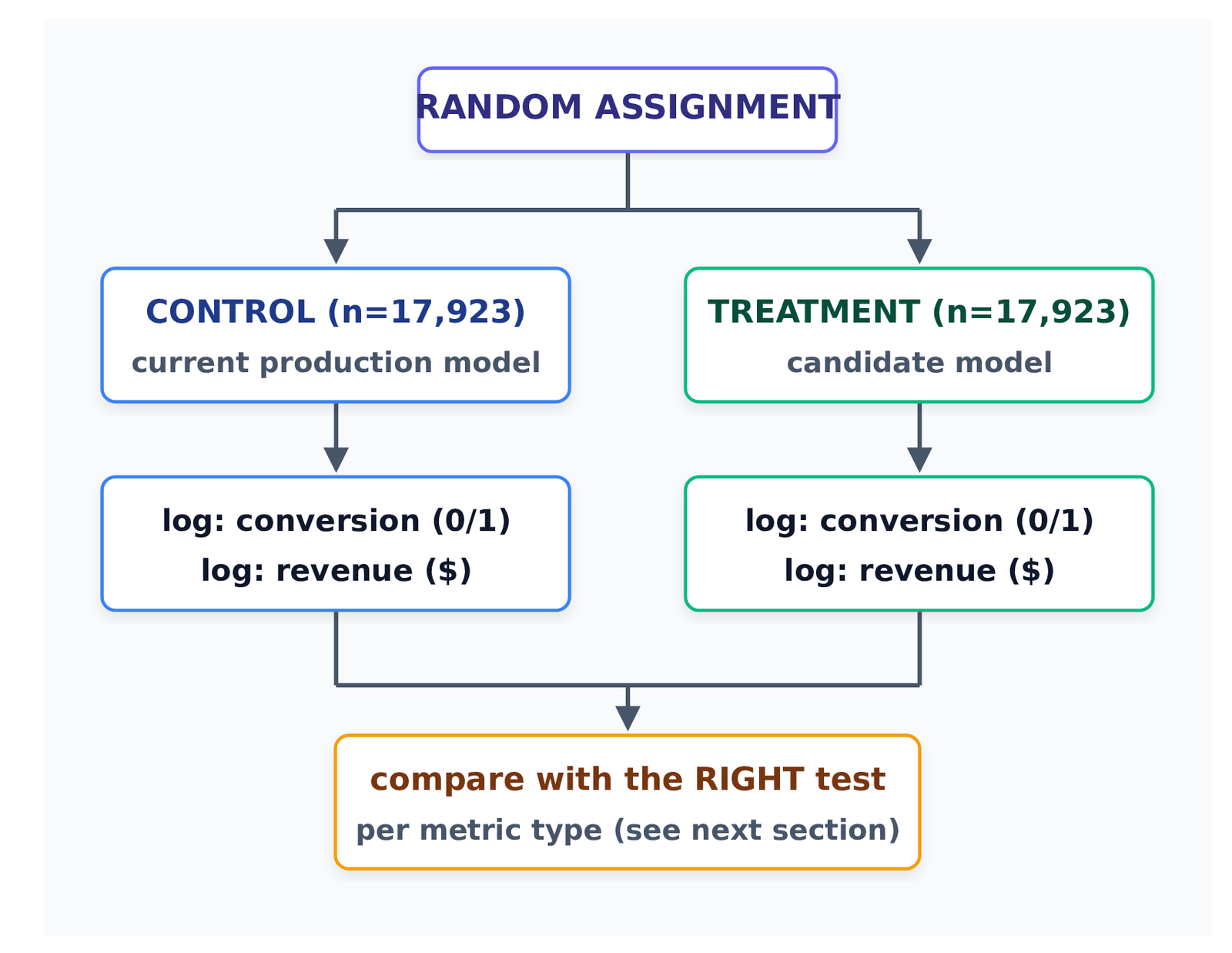
Control is the model currently in production. Treatment is the candidate. Users get randomly assigned to one or the other, and the assignment has to happen before either model is invoked, not after, or you contaminate the comparison with selection bias.

The metric selection matters as much as the model does. In the simulation below, I tracked two: a primary metric, conversion (did the user take the target action), and a secondary metric, revenue per user. Conversion is a proportion — each user is a 0 or a 1, and a two-proportion test applies cleanly. Revenue is continuous, right-skewed, and zero-inflated — about 96% of simulated users spend nothing, and the rest follow a lognormal spend distribution. Those two metrics need two different statistical tools, which is the subject of the next section.

Here’s the actual assignment and outcome from one run, control simulated at a true 4.00% conversion rate, treatment simulated at a true 4.60% rate (a genuine, deliberately-planted 15% relative lift):

Arm	Users	Conversions	Observed rate
Control	17,923	692	3.861%
Treatment	17,923	814	4.542%

Observed relative lift came out to 17.63%, a bit above the 15% I planted, which is just sampling noise at this size — expected, not a red flag. The point of simulating a known ground truth is that I can say with certainty whether the test’s conclusion was correct, and here it was: p=0.0013, clearly below 0.05.

One design decision worth calling out explicitly: decide your primary metric, your guardrail metrics, and your minimum detectable effect before the experiment starts, not after you’ve seen a few days of data. Everything in the “Handling Multiple Metrics” and “5 Common Mistakes” sections below is what goes wrong when that order gets reversed.

Statistical Significance for ML Experiments (Without a Stats Degree)

For a proportion metric like conversion, the right tool is a two-proportion z-test. It compares two observed rates against the standard error of their difference, and it’s what produced the p=0.0013 result above.

For a continuous, skewed metric, it’s tempting to run the same kind of t-test and call it done. I did exactly that on the revenue data, same sample size, same experiment:

	Mean	Median	Skew
Control	$1.3740	$0.00	13.85
Treatment	$1.3907	$0.00	15.75

Welch’s t-test on that: t=-0.1482, p=0.8822. Not significant. I didn’t stop there, because a t-test’s p-value on heavily skewed data can be misleading in either direction, so I ran a bootstrap on the same two samples instead — resample both arms 10,000 times with replacement, take the difference in means each time, and look at where the resulting distribution actually sits.

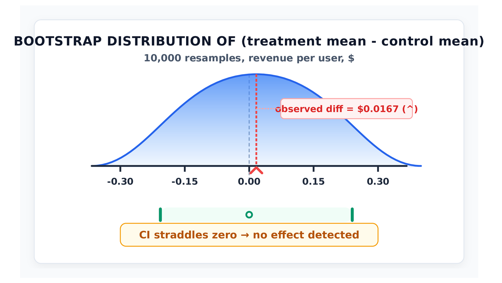
The bootstrap agreed with the t-test: 95% CI of [-$0.2069, $0.2400], straddling zero, two-sided bootstrap p-like value of 0.8876. Both methods landed on the same answer here, which is itself the finding worth reporting — the sample size that comfortably powers a 4% conversion metric can leave a noisier revenue metric with no real signal at all, even when a genuine lift exists somewhere upstream. If you only run the test that matches your primary metric and never check whether your secondary metrics were adequately powered for the same N, you won’t know this happened.

Rule of thumb: match the test to the metric’s actual distribution. Proportions get a proportion test. Skewed continuous metrics get a bootstrap alongside (not instead of) a t-test, and if they disagree, believe the bootstrap.

Handling Multiple Metrics and Conflicting Signals

Real ML experiments rarely track one metric. Conversion, revenue, latency, and a couple of guardrail metrics is a normal set. Each additional metric checked at α=0.05 adds its own 5% chance of a false alarm, and those chances compound.

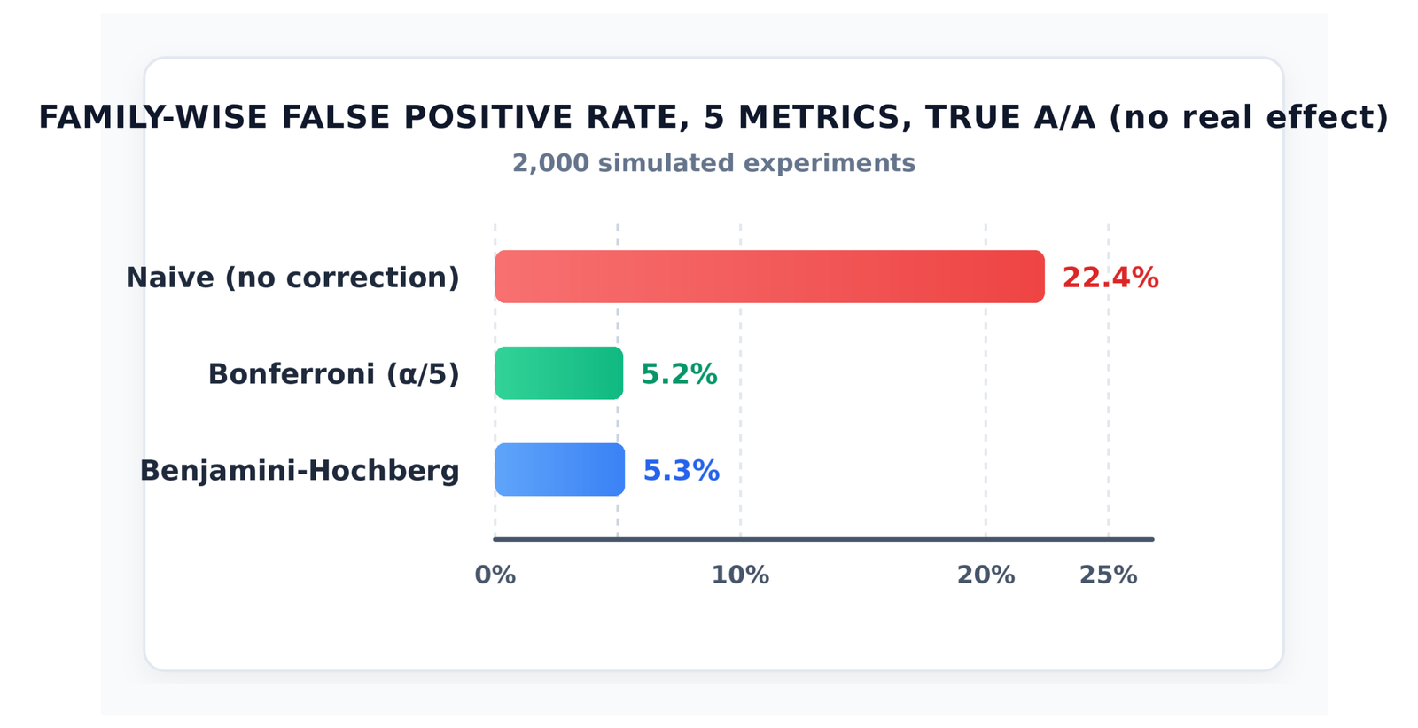
I tested this directly rather than citing the theory and moving on. Simulated a true A/A test — control and treatment statistically identical, no real effect anywhere — across 5 metrics, repeated 2,000 times:

Correction method	Family-wise false positive rate
None (naive α=0.05 per metric)	22.4%
Bonferroni (α/5 = 0.01)	5.2%
Benjamini-Hochberg (FDR)	5.3%

22.4% lines up almost exactly with the textbook prediction, 1-(0.95)^5 = 22.6%. That’s not a rounding coincidence — it’s confirmation the simulation is doing what the underlying probability theory says it should when several independent significance tests are run at once, the chance that at least one comes back significant by chance climbs well above the per-test rate, a point first formalized for the multiple-comparisons case by Bonferroni-style corrections and later generalized in the false discovery rate framework introduced by Benjamini and Hochberg as a less conservative alternative to controlling the probability of any single false positive.

Bonferroni is the blunt instrument: divide α by the number of metrics, and test each one against the smaller threshold. It brought the family-wise rate down to 5.2% here, right where it should land, at some cost in power for a real effect that’s borderline. Benjamini-Hochberg is close behind at 5.3% but controls a different quantity — the expected proportion of false positives among the metrics you call significant, not the probability of any single false positive — which makes it the better default in practice when you have several correlated secondary metrics and don’t want Bonferroni’s full conservatism.

Practical version: decide your primary metric before the experiment. Everything else is a guardrail, tested with a correction applied, not treated as a second chance to find a win.

How Long Should You Run an ML A/B Test?

This is a power analysis question, and the answer depends heavily on your baseline rate, your minimum detectable effect (MDE), and how much traffic you actually have. I ran the calculation for a 4% baseline conversion rate, α=0.05, power=0.80, at 2,500 users per arm per day:

MDE (relative)	Treatment rate	N per arm	Days to run
5%	4.20%	154,283	62
10%	4.40%	39,455	16
15%	4.60%	17,923	8
20%	4.80%	10,297	5
30%	5.20%	4,765	2

The jump from a 5% MDE to a 30% MDE cuts the required sample by over 32x. Small effects are expensive to detect reliably, and that cost grows fast, not linearly — this is the table to show a stakeholder who wants to detect a 3% lift in a two-day test.

Alpha and power also move the number, at a fixed 15% MDE:

α	Power	N per arm	Days
0.05	0.80	17,923	8
0.05	0.90	23,994	10
0.01	0.80	26,669	11
0.10	0.80	14,117	6

Tightening α from 0.05 to 0.01 (fewer false positives allowed) costs almost as much sample size as raising power from 0.80 to 0.90 (fewer missed real effects allowed). Neither is free, and picking both aggressively at once compounds the cost.

The number that matters isn’t “N per arm” in isolation — it’s N per arm divided by your actual daily traffic, which is what turns a sample-size requirement into a commitment on the calendar. An 8-day test is a very different ask from a 62-day one, and running the calculation before the experiment starts is what lets you catch that early, rather than three weeks into a test that was never going to reach significance on the traffic you have.

5 Common Mistakes in ML A/B Testing

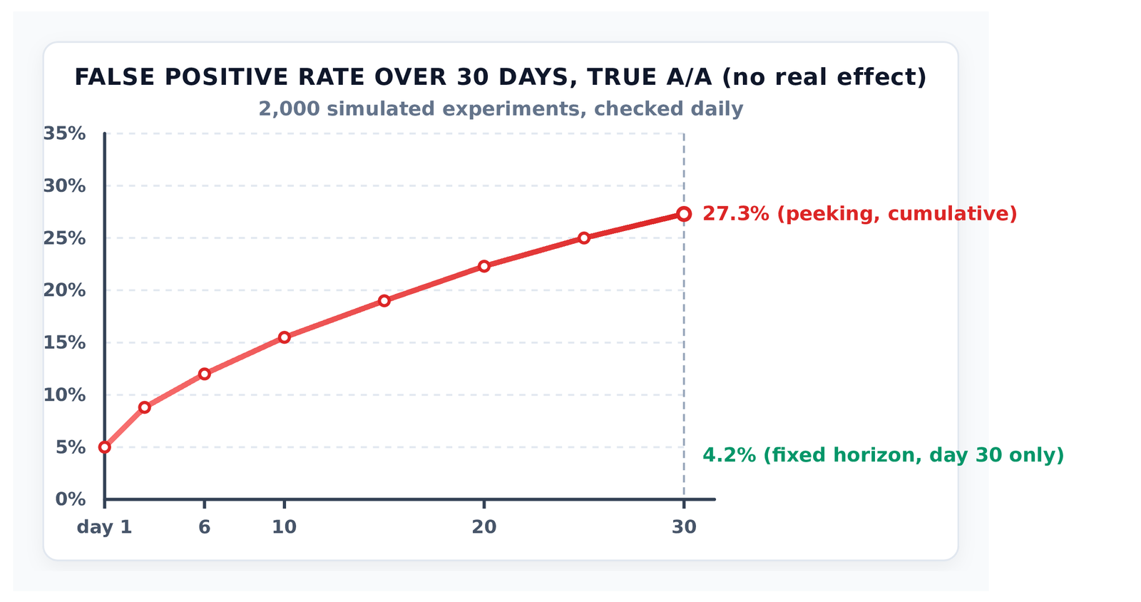
1. Peeking at the results and stopping early. This is the single biggest inflator of false positives I tested, and the numbers are stark. I simulated a true A/A test — no real effect, ever — checked daily for 30 days, at 300 users per arm per day, repeated across 2,000 simulated experiments:

Monitoring approach	False positive rate
Fixed horizon (check once, day 30)	4.2%
Daily peeking, stop at first p<0.05	27.3%

Of the simulations that hit a false p<0.05 at some point, the median day it happened was day 6 — not day 25 or day 29, day 6, with two-thirds crossing within the first 10 days. Checking a live dashboard every morning and stopping the moment it turns green is close to a coin flip on a false win, when there’s no real effect to find. This is the optional stopping problem, and it’s the exact scenario that motivated sequential and “always valid” testing methods designed to let you peek safely by using confidence sequences that remain statistically valid no matter when or how often the experimenter chooses to look at the data. If your organization wants to monitor daily, use a sequential testing method built for it, not a fixed-horizon test checked on a loop.

2. Trusting a mean on a skewed metric. The revenue simulation above used both a t-test and a bootstrap and they agreed — but they don’t always. On a metric with a skew coefficient above 13, a single unlucky or lucky run can shift the mean noticeably without the underlying distribution actually changing. Check the median and the skew alongside the mean before trusting either test’s p-value.

3. Ignoring Sample Ratio Mismatch. Covered in full below — the short version is that a broken 50/50 split can produce a result that looks like a real effect but is actually a logging or assignment bug, and the check for it doesn’t always fire when you’d expect.

4. Under-powering secondary metrics. The N that gives your primary metric 80% power is calculated for that metric specifically. A noisier secondary metric run at the same N, as shown above, can come back with no signal even when a real effect exists — and it’s easy to read that as “no effect on revenue” when the honest read is “this test wasn’t sized to detect it.”

5. Testing five metrics at α=0.05 and calling any winner a win. Covered above — 22.4% family-wise false positive rate with no correction, on data with no real effect at all.

Tools: Statsig, Optimizely, and Custom Implementations Compared

Statsig and Optimizely both provide managed experimentation platforms — sequential testing support, automated SRM checks, and metric dashboards without building the statistical layer yourself. That buys speed and reduces the chance of shipping a peeking bug like the one simulated above. The tradeoff is less control over exactly which test runs on which metric type, and a per-event pricing model that scales with traffic, which matters more once an experiment is running at the kind of volume in the sample-size table.

A custom implementation, the kind built in this article’s five scripts, gives full control over metric-specific test selection (proportion test for conversion, bootstrap for skewed revenue), custom correction methods, and zero per-event cost — at the cost of building and maintaining the statistics layer, including its own tests, which is what test_ab_testing.py in the repo is doing.

	Statsig / Optimizely	Custom (this repo)
Sequential testing / peeking safety	Built in	Must implement (not done here — fixed horizon only)
SRM detection	Built in, automated	Must implement (done here — see below)
Multiple-metric correction	Platform-dependent	Full control (Bonferroni/BH shown above)
Cost model	Per-event pricing	Engineering time, not per-event
Best fit	Teams that want speed over control	Teams already running their own ML infra

Neither option removes the need to understand what’s actually happening statistically — a managed platform running the wrong test on a skewed metric is still running the wrong test. The value of building it yourself once, even if you later move to a managed tool, is that you stop trusting a dashboard’s green checkmark by default.

Sample Ratio Mismatch: The Check That Doesn’t Always Catch What You’d Expect

A Sample Ratio Mismatch (SRM) check asks a simple question before you trust any result: did the traffic actually split the way you configured it? A statistically significant deviation from the intended traffic ratio is treated as a strong warning sign that something is wrong with the experiment’s execution, regardless of what the treatment effect looks like. I ran a chi-square goodness-of-fit test across a few scenarios.

A clean 50/50 split at 40,000 users passed with no issue: p=0.9203. Then I simulated a realistic bug — 1% of treatment-arm events silently dropped before logging, the kind of thing that happens when a slightly slower treatment page causes a few users to bounce before the analytics call fires. At 40,000 users, that 1% drop did not trip a p<0.01 alarm: p=0.443. I pushed the drop rate and the scale to see where detection actually kicks in:

N	Drop rate	Observed ratio	p-value	Detected?
40,000	1.0%	0.4996	0.884	No
40,000	2.0%	0.4950	0.046	No
40,000	3.0%	0.4929	0.005	Yes
200,000	1.0%	0.4979	0.066	No
500,000	0.5%	0.4990	0.167	No
500,000	1.0%	0.4967	<0.001	Yes

A small drop rate at moderate scale can sit right under the detection threshold. This isn’t a flaw in the chi-square test — it’s doing exactly what it’s supposed to do, and a 1% mismatch genuinely produces a small effect on the ratio. The honest takeaway is that an SRM check is a floor, not a guarantee: run it every time, but don’t treat a passing check as proof the logging pipeline is clean, especially on a test that’s smaller or shorter than the ones simulated here.

A/B Testing Machine Learning Models FAQ

Key Takeaways

Match the statistical test to the metric, not the other way around. A proportion gets a proportion test; a skewed continuous metric gets a bootstrap alongside a t-test, and you believe the bootstrap when they disagree.

Sample size that powers your primary metric doesn’t automatically power a noisier secondary one — confirmed directly on simulated revenue data above, where a real underlying lift still came back as “no significant effect” at the same N.

Multiple metrics need a correction. 22.4% family-wise false positive rate with none, brought back to roughly 5% with either Bonferroni or Benjamini-Hochberg, on data with no real effect anywhere.

Peeking is the costliest mistake tested here. 4.2% false positives at a fixed horizon versus 27.3% with daily peeking — both on a true null — and most of the false wins showed up within the first ten days.

An SRM check is necessary, not sufficient. It caught a 3% drop rate at 40,000 users and a 1% drop rate at 500,000, but missed a 1% drop rate at 40,000 users entirely. Run it every time, and don’t over-trust a pass on a small or short test.

What’s Next

A model that wins its A/B test and gets promoted safely is still running on whatever pipeline and infrastructure got it there — and that infrastructure accumulates cost the same way code does. Article 14 covers ML technical debt: the eight types identified in Google’s original technical debt paper, how to audit a system for it, and a scoring framework for deciding what to pay down first. If a test surfaces a model that needs retraining before its next rematch, that’s covered in Article 08’s retrain-vs-fine-tune framework. See the Production ML Engineering guide for how the full series connects.

References

[1] Bonferroni, C. E. (1936). Teoria statistica delle classi e calcolo delle probabilità. Publicazioni del R Istituto Superiore di Scienze Economiche e Commerciali di Firenze.

[2] Benjamini, Y., & Hochberg, Y. (1995). Controlling the false discovery rate: A practical and powerful approach to multiple testing. Journal of the Royal Statistical Society: Series B, 57(1), 289-300. https://doi.org/10.1111/j.2517-6161.1995.tb02031.x

[3] Johari, R., Koomen, P., Pekelis, L., & Walsh, D. (2017). Peeking at A/B tests: Why it matters, and what to do about it. KDD 2017. https://doi.org/10.1145/3097983.3097992

[4] Fabijan, A., Gupchup, J., Gupta, S., Omhover, J., Qin, W., Vermeer, L., & Dmitriev, P. (2019). Diagnosing sample ratio mismatch in online controlled experiments: A taxonomy and rules of thumb for practitioners. KDD 2019. https://doi.org/10.1145/3292500.3330722

[5] Kohavi, R., Tang, D., & Xu, Y. (2020). Trustworthy Online Controlled Experiments: A Practical Guide to A/B Testing. Cambridge University Press.

[6] Wald, A. (1945). Sequential tests of statistical hypotheses. Annals of Mathematical Statistics, 16(2), 117-186. https://doi.org/10.1214/aoms/1177731118

[7] Emmimal P Alexander. (2026). How to Debug ML Inference Latency and Throughput Issues. EmiTechLogic, Article 12 of the Production ML Engineering series. https://emitechlogic.com/debug-ml-inference-latency/

[8] Emmimal P Alexander. (2026). Shadow Deployment and Canary Testing for Machine Learning Models: A Practical Guide. EmiTechLogic, Article 11 of the Production ML Engineering series. https://emitechlogic.com/shadow-deployment-and-canary-testing-for-machine-learning-models-a-practical-guide/

Disclosure

All code in this article — the power calculator, the significance testing script, the multiple-metrics simulation, the peeking simulation, the SRM checker, and the 5-test suite — is my own work. No pretrained weights, no external datasets: every experiment is a simulation with a known, planted ground truth, which is what makes it possible to state plainly when a given test got the right or wrong answer. Built on NumPy, SciPy, and statsmodels, all open-source.

Every number here — the sample-size table, the significance test results, the multiple-testing simulation, the peeking simulation, and the SRM table — came from real runs on Python 3.12.3, NumPy 2.4.4, SciPy 1.17.1, statsmodels 0.14.6. Seed 42 throughout. Re-run independently on a separate Windows machine during review; every figure matched exactly, including the resampling-heavy multiple-testing and peeking simulations, confirming the numbers aren’t an artifact of one environment. Total script runtime varied by hardware (27s on one machine, 111s on another) and that variance is reported rather than smoothed into a single misleading number.

No affiliate relationships. Statsig and Optimizely are discussed based on publicly documented product capabilities, not sponsorship. All comparisons are my own independent evaluation.

This is Article 13 of the Production ML Engineering series. Article 12: How to Debug ML Inference Latency and Throughput Issues covers the performance work that typically precedes a model being ready for this kind of test.