
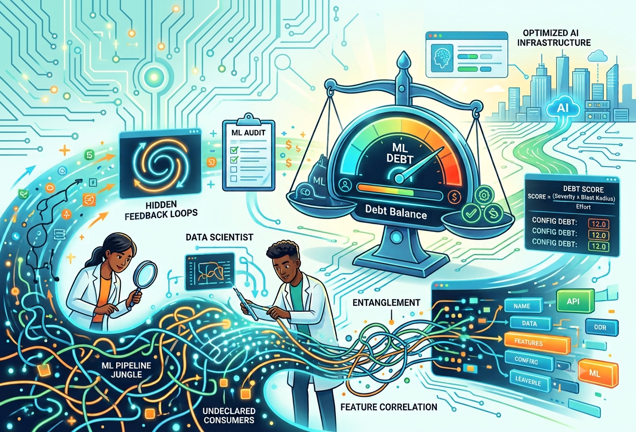
ML Technical Debt: How to Identify, Measure, and Pay It Down
Technical debt in a normal code base is a metaphor. In an ML system, however, it’s closer to a physical description. The debt doesn’t sit quietly in a file waiting for someone to get around to it. Instead, it actively reshapes what a model does while it’s still live, still scoring real traffic, because nobody has to touch the code at all. That’s the central claim of Sculley et al.’s 2015 paper, and more than a decade later, most of what it describes still holds up against real production systems.
This article runs three of that paper’s debt categories through actual code. Rather than retelling the paper’s own examples, it uses new simulations built to reproduce the same failure modes, plus a small static-analysis tool built from scratch to catch two of them mechanically. The most counterintuitive result: dropping a correlated feature and retraining barely moves what the model predicts, while it quietly rewrites which features get the credit underneath. That gap between “predictions look fine” and “the model changed” is where most of the danger in this article lives. Everything below ran on Python 3.12.3, NumPy 2.4.4, scikit-learn 1.8.0, pandas, and pytest, with seed=42 wherever randomness is involved. Every script, the sample repo used for the audit (before and after refactor, plus a deliberately broken version), and the raw output are linked in the Resources section at the end.
Want to reproduce the numbers yourself? Clone the companion repository linked in Resources & References and run
python run_all.py. It executes all six scripts in the order this article presents them and prints every number quoted below. https://github.com/Emmimal/ml-technical-debt-code/
TL;DR
- Dropping one feature from a correlated set and retraining shifted the other features’ learned coefficients by 110.1% on average, versus 10.5% for the identical operation on independent features. Predictions, however, moved the opposite direction: less under correlation than under independence. That’s the opposite of what “entanglement” sounds like it should do, and the actual reason it’s dangerous.
- A purely greedy recommender locked onto 12 of 200 items and never showed anything else across 60 rounds and 30,000 simulated users. Its 10 most-shown items had 0/10 overlap with the true top-10 by quality.
- A characterization test caught a one-line “simplification” that silently changed 58.68% of one column’s values, turning 2,934 rows into NaN with zero errors thrown, exactly the kind of change a code review alone would wave through.
The article also covers a ~100-line static auditor that catches undeclared consumers and configuration debt mechanically, and a severity x blast-radius / effort scoring framework that ranks the cheapest fix above the two flashier findings once cost gets factored in. Full numbers for both are below.
What Is Technical Debt in Machine Learning? (It Is Not Just Code)
Ordinary software technical debt has a fairly fixed shape. Someone took a shortcut, so the code got uglier or more duplicated than it should be. As a result, the team pays interest on that later, in the form of slower changes and more careful reviews. Because the shortcut is right there in the diff, you can usually spot it just by reading the code.
ML technical debt includes all of that, plus a category that doesn’t live in the code at all. That’s because a model’s behavior is a function of its training data, the other features it was trained alongside, the systems it’s coupled to downstream, and the world it’s making predictions about. Every one of those can drift, correlate, or start feeding on its own output without a single commit landing. That’s exactly why Sculley et al.’s 2015 paper, “Hidden Technical Debt in Machine Learning Systems,” matters: it turns a vague unease every ML team eventually develops into an actual checklist [1]. Its central claim is blunt: treating a fast, working ML system as free is a mistake, because it accrues debt through channels that are invisible to the code-review process that catches ordinary debt.
The term itself is older. Ward Cunningham coined “technical debt” in 1992 to describe the tradeoff between shipping fast now and paying interest on messy code later [2]. What the 2015 paper adds, however, is the observation that ML systems have several extra ways to go into debt that have nothing to do with code quality. Three of those get demonstrated here with real numbers instead of just described.
The 8 Types of ML Technical Debt from the Google Paper, Explained
The paper’s own grouping covers boundary erosion and entanglement, correction cascades, and undeclared consumers. It also covers data dependencies (both unstable and underutilized), feedback loops (direct and hidden), and configuration debt. Rounding it out: changes in the external world, plus a family of system-level anti-patterns that includes glue code, pipeline jungles, and dead experimental paths [1]. Most summaries compress that into “8 types,” which is the framing used here. Entanglement, hidden feedback loops, and undeclared consumers/glue code are each demonstrated below on code that actually ran, not just cited.
Entanglement: When Changing One Feature Breaks Everything
The paper’s shorthand for entanglement is CACE (Changing Anything Changes Everything). In a cleanly interfaced system, you can usually reason about a change’s blast radius by reading the function signature. A jointly-trained ML model, however, doesn’t give you that. Because it doesn’t treat features as independent inputs, it treats them as whatever combination best explains the training labels. So if two features carry overlapping signal, the model has no concept of which one “should” get credit for it.
The setup: a logistic regression trained on 10 features, under two conditions. In the CORRELATED condition, all 10 features load onto two shared latent factors plus noise, which is a reasonable stand-in for an engineered feature set. For example, half the columns might be ratios, rolling aggregates, or counts derived from the same handful of raw events, which describes most production feature stores. In the INDEPENDENT condition, by contrast, the 10 features are statistically unrelated to each other. Everything else stays identical: same label-generating process, same sample size (20,000 rows, 70/30 split), same model (regularized logistic regression, C=1.0), seed=42 in both.
The experiment: remove one feature entirely (a routine deprecation, a vendor field that stops sending data, a raw signal getting retired) and retrain from scratch. Then measure how far the remaining features’ learned weights move, and how far the model’s predictions on a fixed holdout set move too, even though nothing about those remaining features changed on disk.
| Condition | Mean absolute coefficient shift on remaining features | Mean absolute predicted-probability shift |
|---|---|---|
| Correlated features | 110.1% | 0.0323 |
| Independent features | 10.5% | 0.0849 |
Coefficient shift is calculated as mean(abs(new_coef – old_coef) / abs(old_coef)) across the nine surviving features, expressed as a percentage. Prediction shift is the mean absolute probability difference between the two models’ outputs on the same fixed holdout set.
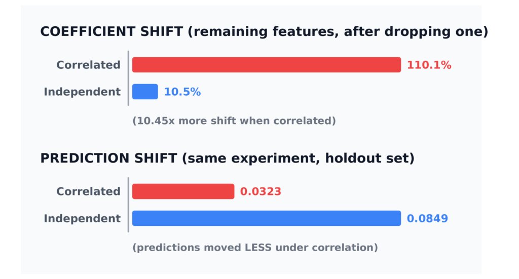
The first row is the expected result. With correlated features, dropping one moved the other features’ weights by 110% on average, more than doubling in either direction, for a change that had nothing to do with them directly. Independent features, by comparison, moved about a tenth as much for the identical operation. That’s a concrete example of the CACE effect described in the paper.
The second row is the part worth sitting with, because it inverts the intuition. Predictions were more stable under correlation, not less: a 0.032 average shift versus 0.085 under independence. That isn’t a contradiction, though. It’s the actual mechanism. Because features are correlated, whichever ones survive the drop can absorb the missing feature’s signal, so the model keeps performing about as well as it did before. What changes instead is the internal attribution: which feature the model is leaning on, and how hard. That shift happens completely underneath a nearly-unchanged accuracy number.
That’s the practical danger. Because the thing that moved isn’t the thing those detectors watch, a monitoring dashboard that watches only accuracy or AUC (the kind built in Article 9 of this series) may not flag this. So anything downstream that depends on feature importance goes stale the moment one correlated feature gets touched. Think an explainability report, a fairness audit segmented by which features drive which predictions, or a regulatory filing describing how the model works. It happens silently, and the accuracy metric gives no warning at all.
Hidden Feedback Loops in Production ML
A hidden feedback loop happens when a model’s own output shapes the data it will be trained on next, through some indirect path. For example, a user can only click on what they were shown, and an ad system can only learn from impressions it chose to serve. The paper’s example is a news recommender that starts favoring certain stories. Because those stories are what’s in front of them, users click those. The system then reads the clicks as proof those stories work, so the loop tightens on itself [1].
The simulation: 200 items, each with a true latent quality score drawn from a Beta(2, 5) distribution. This creates a skewed catalog in which most items have relatively low latent quality and only a handful are genuinely good. Each round, 500 simulated users arrive, and the system recommends its current top-10 by estimated quality. Users then engage probabilistically according to the item’s true quality, and those engagement counts update the estimate for the next round. Two policies run head to head, same seed, same starting prior. GREEDY always shows the current top-10 by estimate. An epsilon-greedy EXPLORING policy, however, swaps in a couple of items from outside the current top-10 each round. That’s 15% of the recommended slots, chosen at random from what greedy would have excluded.
Run for 60 rounds, 30,000 simulated users total:
| Metric | Greedy | Exploring (15%) |
|---|---|---|
| Gini coefficient, round 1 | 0.950 | 0.950 |
| Gini coefficient, round 10 | 0.950 | 0.943 |
| Gini coefficient, round 30 | 0.950 | 0.923 |
| Gini coefficient, round 60 | 0.950 | 0.901 |
| Items that ever got shown (of 200) | 12 | 66 |
| Overlap with the true top-10 by quality | 0 / 10 | 2 / 10 |
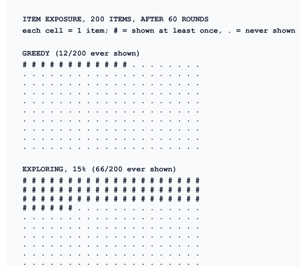
The grid isn’t mapping specific item IDs to specific cells. It’s a proportional visualization instead, showing how much of the catalog either policy actually explored. The counts behind it are exact, though: 12 of 200 for greedy, 66 of 200 for exploring, straight from the simulation log.
The Gini coefficient staying flat at 0.950 for greedy across all 60 rounds isn’t a sign that nothing happened. It’s the opposite. The greedy policy concentrates exposure from the beginning, leaving 188 of the 200 items with zero exposure in this run. Whatever ranked in the top-10 before any real engagement signal existed is what the system decided was “good,” so the initial ranking receives most of the system’s subsequent evidence, and from then on it only ever collected evidence in favor of its own initial guess.
The overlap number is the one to sit with longest. After 60 rounds and 30,000 users, greedy’s 10 most-shown items had 0/10 overlap with the true top-10 by quality. The system wasn’t broken because its logic was bad; “show what performed well” is completely sound reasoning in isolation. Instead, it failed because the only data it ever collected was about the items it had already decided to show, so it could never discover that something better existed outside that set. Exploration didn’t eliminate the problem, but it did visibly dent it: 66 items got some exposure instead of 12, and 2 of the true top-10 surfaced instead of 0. That’s a real, measurable performance cost in the short run, paid in exchange for a system that can still learn something it doesn’t already believe. This is the same tradeoff that motivated the multi-armed-bandit literature on exploration versus exploitation more broadly. The specific failure mode here, recommender feedback loops narrowing a catalog’s effective diversity over time, also has its own dedicated research thread outside the original debt paper [3].
Undeclared Consumers and Pipeline Glue Code
An undeclared consumer is any system reading an artifact (a shared table, a feature file, a model binary) without the artifact’s owner knowing that consumer exists. There’s no interface, no schema contract, no version agreement between them. As a result, it’s one of the most ordinary ways an “innocent” change breaks something nobody remembered depended on it: a column rename, a threshold update, a field getting retired.
This category doesn’t need a simulation, because it’s visible from the code as written. That’s exactly why it’s demonstrated with a scanner instead. The scanner runs against a small 5-file sample pipeline built to resemble a typical evolved ML repo: a feature-generation script, a training script, a batch-scoring script, a Flask serving API, and a legacy orchestration script that chains the others together with subprocess calls and file copies. In other words, a pipeline jungle in miniature, on purpose.
The scan found data/features.csv referenced directly, by literal path string, in 4 separate files: the script that writes it, plus 3 more that each independently decided to read it. Similarly, two model artifacts (model_v3_final_FINAL.pkl and scaler_v3.pkl) were each read directly by 3 files, and a data/scores_output.csv was shared by 2. None of these five had an interface, a version tag, or a schema check anywhere between writer and reader. That’s undeclared consumption exactly as the paper describes it: cheap to create, invisible until the day the writer changes something. When that day comes, three other files break for reasons none of their own authors could see from their own code.
How to Audit Your ML System for Technical Debt
The undeclared-consumer and configuration-debt findings above came from a small, dependency-free static auditor: under 100 lines of Python, using only the standard library’s ast module, no third-party tooling required. This is intentionally a heuristic detector, not a complete dependency analyzer; it can miss things like dynamically constructed paths (Path(DATA_DIR) / filename), and it can flag strings that merely resemble artifact paths without actually being one. It does two things.
First, it walks every .py file in a target directory with ast.parse and collects every string-literal constant that looks like a shared data artifact. That means a path ending in .csv, .json, .pkl, or .parquet, or one starting with data/, models/, archive/, or logs/. Those literals get grouped by exact value. Any literal that shows up in more than one file gets flagged, because those files are coupled to each other through a string. Nothing enforces that the shape of the artifact behind it hasn’t changed between them.
Second, it walks the same files for numeric constants embedded directly in a function call or assignment, excluding any file that’s clearly meant to be config, named config.py or settings.py. It counts the constants per file, leaving out trivial values like 0, 1, and -1 that are rarely “configuration” in intent.
Run against the sample repo, before and after a refactor built specifically to answer these two findings:
| Check | Before refactor | After refactor |
|---|---|---|
| Shared artifacts referenced directly by 2+ files | 4 | 0 |
| Total undeclared-consumer file references | 12 | 0 |
| Configuration debt (magic numbers outside config) | 13 | 3 |
The “after” column is the result of two changes. First, introducing a single feature_store.py module with one declared get_features() function as the only sanctioned way to read the shared data. Second, moving every threshold, split ratio, and hyperparameter into a config.py module that every other file imports from. Because ownership of the raw path was moved behind the feature-store interface, no artifact was directly referenced by multiple files anymore, and the undeclared-consumer count dropped to exactly zero. The configuration-debt count, however, didn’t reach zero: the audit still found 3 remaining magic numbers, one of them a hardcoded port number (app.run(port=5000)) in the serving script that the refactor genuinely missed. That’s worth keeping in the write-up, since an audit tool that reports a spotless pass right after “the big refactor” isn’t measuring anything. It’s just agreeing with whoever ran it. This one still found something, which is closer to what an honest audit should do.
The tool makes no attempt to catch entanglement or feedback loops, because those aren’t visible from static structure. That’s exactly why they needed simulations instead of a scanner. A realistic process, therefore, runs the static scanner on a schedule, since it costs almost nothing to run. It then treats entanglement and feedback-loop risk as something a team reasons about deliberately, on a slower cadence. That’s the same way the two simulations above were built, to make that reasoning concrete instead of a vague sense that something might be wrong.
A Scoring Framework for Prioritizing Debt Reduction
Once an audit turns up eight or ten findings spread across four different debt categories, “fix whatever sounds scariest first” is a weak prioritization method. That’s because how alarming a finding sounds has very little to do with its actual cost-to-fix ratio. The framework used here is deliberately simple:
Debt score = (Severity x Blast Radius) / Effort
Severity and effort are both judgment calls on a 1-5 scale, made by whoever actually understands the system. Severity is how bad the failure mode gets if the debt bites. A silent wrong prediction, for instance, ranks above slow iteration speed, which in turn ranks above code that’s merely ugly. Effort is a rough cost estimate: 1 means moving a value into a config file, while 5 means a genuine re-architecture. Blast radius is capped on the same 1-5 scale, and that cap is deliberate. Raw audit counts, after all, are in completely different units from each other. A 200-item catalog, for example, dwarfs a 4-file coupling every time as a raw number. If the raw count set the score directly, whichever finding happens to have the biggest denominator would win the backlog, for a reason that has nothing to do with actual priority. So the audit’s count still decides where a finding lands on the 1-5 scale, but it doesn’t get to set the scale itself.
One caveat worth stating plainly before the table below: severity and blast radius are engineering judgment calls, made by whoever triages the finding, not experimentally measured physical quantities. What the arithmetic buys you is a reproducible, arguable ranking, not an objective one. Two engineers who disagree on a severity rating will still get a consistent answer once they agree on the inputs. That’s the actual value here, not false precision.
Applied to every finding surfaced above:
| Score | Category | Severity | Blast Radius | Effort | Finding |
|---|---|---|---|---|---|
| 12.0 | Configuration debt | 3 | 4 | 1 | 13 magic numbers outside config |
| 10.0 | Undeclared consumers | 5 | 4 | 2 | features.csv read directly by 4 files |
| 8.3 | Hidden feedback loop | 5 | 5 | 3 | Greedy recommender: 12/200 shown, 0/10 true-best overlap |
| 6.7 | Entanglement (CACE) | 5 | 4 | 3 | Correlated features: 110% coefficient shift on feature drop |
| 6.0 | Undeclared consumers | 4 | 3 | 2 | model_v3_final_FINAL.pkl read directly by 3 files |
| 6.0 | Undeclared consumers | 4 | 3 | 2 | scaler_v3.pkl read directly by 3 files |
| 4.5 | Glue code / pipeline jungle | 3 | 3 | 2 | Legacy script chains stages via subprocess + file drops |
| 4.0 | Undeclared consumers | 2 | 2 | 1 | scores_output.csv read directly by 2 files |
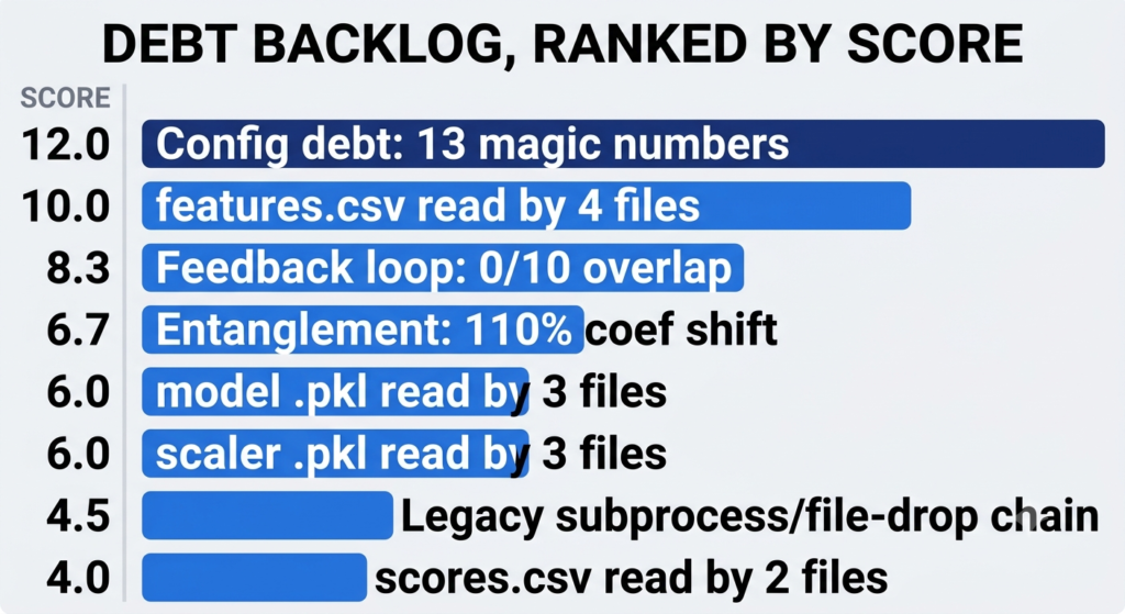
The config-debt cleanup comes out on top, not the entanglement finding and not the feedback loop, even though those two produced by far the most dramatic numbers in this article. That’s the actual point of running the arithmetic instead of prioritizing by gut feel. Because config debt is cheap to fix (effort 1) and was assigned a broad blast radius (4), it wins on a cost-adjusted basis, even though “13 magic numbers” doesn’t sound remotely as alarming as “the recommender can’t discover its own best items.” The feedback loop and entanglement findings are real and severe. However, they’re also the most expensive to actually resolve, since fixing either means changing the system’s exploration policy or building explicit dependency tracking into the feature pipeline. Neither is as simple as moving a threshold into a file.
Refactoring ML Code Without Breaking Production
Every fix in the table above means touching code that’s currently running correctly in some sense. Even the entangled model and the greedy recommender are producing usable output today. The risk in refactoring an ML pipeline, therefore, isn’t that the code stops running. It’s that it keeps running and starts silently returning different numbers, so nothing flags it until a downstream consumer notices something’s off, days or weeks after the change shipped.
The safety net demonstrated here is a characterization test. Before touching anything, capture the exact output of the current code on a fixed input as a golden reference. Then, after refactoring, regenerate on the identical input and assert the two match exactly, not an approximate or tolerance-based comparison. This is the same technique Michael Feathers formalized under the term “characterization test.” It fits exactly this situation: legacy code with no spec and no test coverage, where the goal of a first pass isn’t correctness. It’s simply not silently changing what’s already there [4].
Run against the actual before/after refactor from the audit section, the same 5,000-row synthetic input. feature_gen.build_features() (before) against feature_store.build_features() (after). The test passed: the refactored output matched the original exactly, confirmed with pandas.testing.assert_frame_equal(check_exact=True) [5].
A passing result only means something if the same test can also fail. So a second version was built with a deliberately realistic slip: the refactor “simplified” a rolling-average line by dropping a min_periods=1 argument that looked redundant in review. The window size is still rolling(7), so nothing about the call’s intent looks different on the surface. Even so, the characterization test caught it immediately:
DataFrame.iloc[:, 6] (column name="rolling_7d") values are different (58.68 %)
rolling_7d NaN count - before: 0, broken after: 293458.68% of the values in that one column changed, and the count of missing values in it went from 0 to 2,934. That’s because without min_periods=1, the first 6 rows for every user now return NaN instead of a partial-window average. As a result, every downstream consumer of that column would have started silently receiving nulls for a meaningful slice of users. Think the training script, the batch scorer, the serving API’s lookup cache. There would be no crash, no schema change, and no monitoring alert, because nothing about the data types or the pipeline’s shape changed.
The practical rule this produces: any refactor billed as behavior-preserving gets a characterization test first, not a code review alone. A review catches things that look wrong on the page. A characterization test catches things that look completely fine and aren’t.
Preventing Future Debt: Standards, Reviews, and Documentation
Everything above is remediation: finding debt that’s already there and paying it down. The cheaper version of the same work is not accumulating it in the first place. The practices that hold up are unglamorous:
One declared read/write interface per shared artifact, enforced by convention or by making the raw path genuinely hard to reach from anywhere else in the code base. The refactor in this article did exactly this with a single get_features() function. It’s the entire reason the undeclared-consumer count went to zero.
One config module per project, with a habit of asking “does this number belong in config.py” the moment it’s written. It’s cheap at the point of creation, but expensive to retrofit once it’s scattered across a dozen files, which is what the config-debt score above is actually measuring.
A characterization test as a standing requirement before any refactor that touches shared data or a model already serving traffic, not reserved for large changes. The bug caught above came from a one-line edit that looked completely safe in review.
Running the static auditor (or one like it) on a schedule, not just before a big cleanup sprint. This kind of debt accumulates a few lines at a time, so catching it monthly is a fundamentally different job than catching it after eighteen months of quiet growth. It’s the difference between a ten-minute fix and the kind of rewrite that ends up as its own line item on next quarter’s roadmap.
Feeding the audit’s findings into the same scoring framework every time, instead of re-litigating priority from scratch on each pass. The value of (severity x blast radius) / effort isn’t the specific formula. Rather, it’s that it forces severity, effort, and scope to get named out loud, instead of implied by whoever’s most recently annoyed by a given piece of debt.
ML Technical Debt FAQ
What is the Google paper everyone cites about ML technical debt?
“Hidden Technical Debt in Machine Learning Systems,” by D. Sculley and colleagues at Google, published at NeurIPS (then still called NIPS) in 2015 [1]. It introduced entanglement (CACE), hidden feedback loops, undeclared consumers, and several other ML-specific debt categories as a class of problem distinct from ordinary software debt.
Is entanglement the same thing as feature correlation?
Related, not identical. Feature correlation is a property of the data, while entanglement is what that correlation does to a jointly-trained model’s behavior once one of the correlated features changes or disappears. The simulation above shows the same underlying correlation producing a smaller effect on predictions but a larger effect on the model’s internal attribution. That second part is the finding that actually matters for auditing a live system.
Can a static audit tool catch entanglement or hidden feedback loops automatically?
No, not through static analysis alone. The auditor in this article catches undeclared consumers and configuration debt because both are visible directly in the code as written. Entanglement and feedback loops, however, are properties of how a trained model behaves once it’s live, which is why they’re demonstrated here with simulations instead of a scan. A team has to deliberately test for them, the same way you’d test for a security vulnerability rather than expect a linter to find it for free.
Do I need a commercial tool to find undeclared consumers, or does a simple script actually work?
A simple script is sufficient for this narrow class of findings, and it has one advantage a commercial tool doesn’t: it’s fully auditable itself. The scanner used here is under 100 lines of standard-library
astparsing, with no dependencies. Every design decision, what counts as an artifact-like string, what counts as a trivial number, is visible and adjustable, rather than hidden inside a commercial product’s undocumented heuristics.Why does a scoring framework divide instead of just adding severity and blast radius?
Division puts cost directly into the ranking. A severity-5, blast-radius-5 fix that takes one day should clearly outrank a severity-3 fix that takes five days, and
(5*5)/1 = 25versus(3*3)/5 = 1.8gets that ordering right. A flat sum wouldn’t, because it ignores effort entirely unless it’s subtracted in, which just reintroduces the unit-mismatch problem the cap on blast radius already solves.
Key Takeaways
Entanglement doesn’t show up where the name suggests it will. Correlated features produced a smaller shift in predictions than independent features did, for the identical operation. The actual risk sits in the coefficients and the attribution shifting underneath a nearly-unchanged accuracy number, not in the accuracy number itself.
A feedback loop can lock in a wrong answer permanently, starting from the very first round, before any real signal exists to justify it. Under a purely greedy policy, the 10 most-shown items had 0/10 overlap with the true top-10 by quality, across 60 rounds and 30,000 simulated users.
Undeclared consumers and configuration debt are both mechanically detectable with a small static-analysis script. No framework, no paid product. Under 100 lines of ast parsing caught every instance used in this article’s examples.
A scoring framework that caps blast radius on the same scale as severity and effort keeps the backlog honest. The cheapest, broadest-reaching fix outranked the two most dramatic-sounding findings once cost actually got factored in.
A characterization test is the difference between a refactor that’s genuinely safe and one that merely looks safe in review. It caught a one-line change that silently turned 58.68% of a column’s values into something else, with zero errors thrown anywhere.
What’s Next
This picks up right after Article 13’s A/B testing framework, which proves a model candidate is actually better before any of this debt-reduction work becomes relevant to it. Next and last in the series: Article 15, an ML production readiness checklist, which folds this article’s audit tool and scoring framework together with deployment (Article 2), retraining (Article 3), versioning (Article 4), monitoring (Article 10), shadow deployment (Article 11), and latency debugging (Article 12) into one pre-ship checklist. See the Production ML Engineering guide for the full series map.
Resources & References
[1] Sculley, D., Holt, G., Golovin, D., Davydov, E., Phillips, T., Ebner, D., Chaudhary, V., Young, M., Crespo, J.-F., & Dennison, D. (2015). Hidden technical debt in machine learning systems. Advances in Neural Information Processing Systems 28 (NeurIPS 2015), 2503-2511. https://proceedings.neurips.cc/paper/2015/hash/86df7dcfd896fcaf2674f757a2463eba-Abstract.html
[2] Cunningham, W. (1992). The WyCash portfolio management system. OOPSLA ’92 Experience Report. The original description of the technical debt metaphor. https://dl.acm.org/doi/10.1145/157709.157715
[3] Fleder, D., & Hosanagar, K. (2009). Blockbuster culture’s next rise or fall: The impact of recommender systems on sales diversity. Management Science, 55(5), 697-712. Covers how recommender feedback loops narrow effective catalog diversity over time, the phenomenon the greedy-vs-exploring simulation above reproduces at small scale. https://doi.org/10.1287/mnsc.1080.0974
[4] Feathers, M. (2004). Working Effectively with Legacy Code. Prentice Hall. Source of the “characterization test” concept used in the refactoring section above.
[5] pandas development team. pandas.testing.assert_frame_equal documentation. https://pandas.pydata.org/docs/reference/api/pandas.testing.assert_frame_equal.html
[6] Python Software Foundation. ast (Abstract Syntax Trees), Python standard library documentation. Used to build the static auditor with no third-party dependency. https://docs.python.org/3/library/ast.html
[7] scikit-learn developers. sklearn.linear_model.LogisticRegression documentation. https://scikit-learn.org/stable/modules/generated/sklearn.linear_model.LogisticRegression.html
[8] Emmimal P Alexander. (2026). How to A/B Test Machine Learning Models the Right Way. EmiTechLogic, Article 13 of the Production ML Engineering series. https://emitechlogic.com/how-to-a-b-test-machine-learning-models-the-right-way/
[9] Emmimal P Alexander. (2026). How to Debug ML Inference Latency and Throughput Issues. EmiTechLogic, Article 12 of the Production ML Engineering series. https://emitechlogic.com/debug-ml-inference-latency/
Full code, all six scripts (entanglement simulation, feedback-loop simulation, static auditor, scoring framework, and both characterization tests), the sample repo in its before/after/broken states, and the raw run logs quoted above, is available in this article’s companion repository: https://github.com/Emmimal/ml-technical-debt-code/
Disclosure
All code in this article is my own work, built and executed specifically for this piece. That includes the entanglement simulation, the feedback-loop simulation, the static debt auditor, the scoring framework, and both characterization tests (the passing run and the deliberately broken one). There are no pretrained weights and no external or scraped datasets. Every number is either a real simulation with a known, planted ground truth, or the direct output of a static scanner run against a small sample repo built to resemble a typical evolved ML pipeline. It’s built entirely on open-source tooling: NumPy, scikit-learn, and pandas.
Every figure quoted above came from real runs on Python 3.12.3, NumPy 2.4.4, scikit-learn 1.8.0, pandas, and pytest 9.1.1. That covers the entanglement coefficient and prediction shifts, the feedback-loop Gini and overlap numbers, the audit tool’s before/after counts, the scoring table, and both characterization test outputs. Seed 42 throughout, wherever randomness enters the picture.
No affiliate relationships, no sponsorships, and no tool mentioned above (scikit-learn, pandas, pytest) paid for placement. They’re referenced because they’re what the code actually runs on.
This is Article 14 of the Production ML Engineering series.





Leave a Reply