

What Is Big O Notation? Time and Space Complexity Explained
This article is part of the Data Structures & Algorithms with Python roadmap, and it’s the right place to start if you’re new to analyzing code efficiency.
You write a Python function. It works fine on your test data. Then you run it on real data, and it crawls. Nothing crashes. It just takes forever. This happens to almost every developer at some point. The code is correct, but it is slow, and you do not know why. Big O notation is the tool that explains this. It tells you how your code’s speed and memory use change as your input grows, before you ever run it.
This guide is for Python learners, developers preparing for interviews, and anyone who wants to write code that stays fast as data grows. By the end, you will know what Big O means, how to calculate it for your own code, and how to spot the common mistakes people make when they use it.
In Simple Terms
Big O notation describes how the running time or memory use of an algorithm grows as the input size grows. It does not tell you exact seconds or exact bytes. It tells you the shape of growth: does the work stay flat, grow slowly, or explode as input gets bigger?
What Is Big O Notation?
Let’s understand Big O with a simple example.
Imagine you have a phone book with the names of one million people, and you want to find Alice.
Would you start from the first page and check every name one by one?
Probably not.
You would open the phone book somewhere near the middle. If you went too far, you would go back toward the beginning. If you were too early, you would move toward the end. Each time, you are cutting down the number of pages you need to search.
Because you are removing about half of the possibilities each time, you can find Alice in surprisingly few steps — even if the phone book contains a huge number of names.
Now imagine a different situation.
You have a shuffled, face-down deck of cards, and you need to find one specific card.
There is no easy shortcut. You have to pick up the cards one by one and check them.
If the card is near the top, you get lucky.
But if the card is the very last one, you have to check every card.
These are both search problems, but they behave very differently as the amount of data increases.
That’s where Big O notation comes in.
So, what exactly is Big O?
Big O notation is a way of describing how the amount of work an algorithm needs grows as the input becomes larger.
The input size is usually represented by n.
For example, if you have an array containing 100 elements, then:
n = 100
If the array contains 1,000 elements:
n = 1000
Big O helps us answer a very important question:
“What happens to my algorithm when the amount of data becomes really large?”
It focuses on the growth of the algorithm, rather than the exact number of seconds it takes to run.
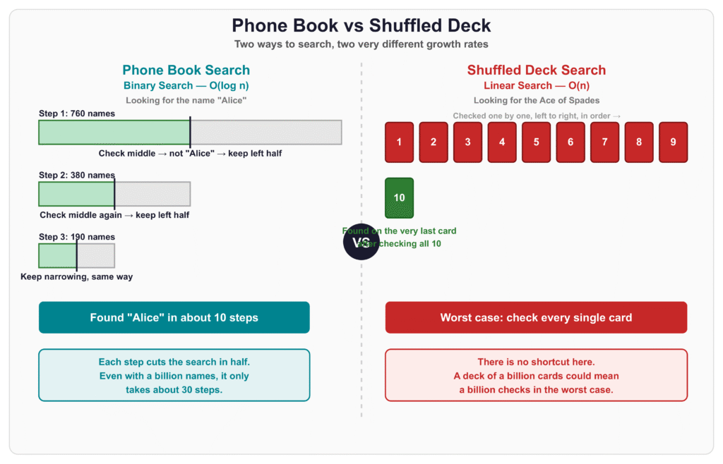
Phone book vs. shuffled deck
The phone book example is similar to binary search.
Every time we look at the middle, we can eliminate roughly half of the remaining possibilities.
This gives us:
O(log n)
The shuffled deck example is similar to linear search.
We may have to check every card, one after another.
This gives us:
O(n)
The phone book example works because the names are arranged in alphabetical order. Without that ordering, you couldn’t simply jump to the middle and eliminate half the search space.
The difference becomes much more important when the amount of data gets larger.
For example, with around one million items:
- O(n) might require checking up to about 1,000,000 items.
- O(log n) requires only around 20 steps when the search space is repeatedly cut in half.
That’s a huge difference.
Big O is about growth, not exact speed
There is an important detail here.
Suppose one algorithm takes 3n operations and another takes n operations.
Both are considered:
O(n)
Why?
Because as n gets larger, both algorithms grow linearly.
Big O is interested in the overall growth pattern, not the exact constant in front of it.
So:
3n → O(n)
100n → O(n)
n + 50 → O(n)
The constants and smaller terms become less important when we are looking at very large input sizes.
Big O is not the same as “worst case”
This is something students often get confused about.
You may hear someone say:
“Big O means worst-case complexity.”
That’s not quite correct.
Big O describes how something grows.
Worst case describes which situation we are analyzing.
These are two different ideas.
For example, when searching through an array:
- The item might be the first element → best case.
- The item might be somewhere in the middle → average case.
- The item might be the last element or not exist at all → worst case.
We can use Big O notation to describe any of these cases.
In practice, however, programmers often talk about the worst-case Big O complexity, because knowing the maximum amount of work an algorithm might require is useful when designing software.
What does Big O ignore?
Big O intentionally leaves out some details.
1. Exact hardware speed
A program might run faster on a powerful computer than on an old computer.
Big O doesn’t care about the exact speed of the computer. It describes how the algorithm’s work grows.
2. Constant factors
As we saw earlier, n, 3n, and 100n are all O(n).
The constant affects actual performance, but it doesn’t change the overall growth pattern.
3. Small inputs
Big O is mainly concerned with what happens when n becomes large.
For a very small input, an O(n²) algorithm might actually run faster than an O(n) algorithm because of differences in implementation and overhead.
The main idea to remember
Don’t try to memorize Big O as a complicated mathematical formula.
Think of it as a way to answer this question:
“As my input gets bigger, how quickly does the amount of work my algorithm has to do grow?”
For example:
O(1) → The amount of work stays roughly the same.
O(log n) → The work grows very slowly.
O(n) → The work grows directly with the input.
O(n²) → The work grows much faster as the input gets bigger.
That’s the basic idea behind Big O notation.
Once you understand this idea, learning how to calculate the Big O of actual code becomes much easier.
Why Big O Matters in DSA
Now that we understand what Big O notation is, you might be wondering:
“Why do we actually need it?”
If an algorithm gives us the correct answer, why should we care about its Big O?
The answer becomes clear when the amount of data gets large.
An algorithm that works perfectly with 10 or 100 items might become extremely slow when it has to deal with 1 million or 100 million items.
This is one of the main reasons Big O notation is so important in Data Structures and Algorithms (DSA).
1. It helps us compare algorithms
Imagine you have two different algorithms that solve the same problem.
One takes O(n) time, while the other takes O(n²) time.
For a small input, you might not notice much difference.
But as the input grows, the difference becomes huge.
For example, if n = 1,000:
- O(n) → about 1,000 units of work
- O(n²) → about 1,000,000 units of work
Both algorithms solve the same problem, but one scales much better than the other.
Big O gives us a simple way to compare them.
2. It helps us choose the right data structure
Data structures are not all good at the same things.
For example, suppose you need to search for a value.
Depending on the situation, you might use an:
- Array
- Linked list
- Hash table
- Binary search tree
Each one can have different performance characteristics.
Big O helps us understand those differences and choose a data structure that fits the problem.
3. It helps us write scalable programs
A program might work perfectly on your computer with a few hundred records.
But what happens when your application has millions of users?
This is where algorithm efficiency really matters.
A poorly chosen algorithm can make an application slow, expensive, or even unusable when the amount of data increases.
By understanding Big O, we can think ahead and choose algorithms that are more likely to handle large inputs efficiently.
4. It helps us identify inefficient code
Big O can also help you look at your own code and ask:
“Is there a better way to do this?”
For example, suppose you have a loop inside another loop.
That might result in O(n²) time complexity.
Sometimes that’s perfectly acceptable.
But if n can become very large, you might look for a way to solve the same problem in O(n) or O(n log n) time.
So Big O isn’t just something you calculate for an exam. It is a way of thinking about the efficiency of your code.
5. It is important for technical interviews
If you are preparing for software engineering interviews, you will almost certainly come across Big O.
Interviewers often ask questions such as:
- What is the time complexity of this code?
- What is the space complexity?
- Can you make this solution more efficient?
- What happens if the input becomes very large?
They aren’t only checking whether you can write code.
They also want to know whether you understand why your solution is efficient.
6. It helps us think beyond “Does it work?”
When you’re learning programming, your first goal is usually:
“Can I make this code work?”
That’s a good starting point.
But DSA takes you one step further:
“Can I make it work efficiently?”
Two algorithms can produce exactly the same result, but one can require dramatically less time or memory.
Big O helps us understand that difference.
A simple example
Suppose you need to find a person’s name in a collection of names.
A simple approach might check every name one by one.
That’s O(n).
But if the data is organized in a way that allows you to repeatedly eliminate half of the possibilities, you might be able to search in O(log n).
Both approaches can find the answer.
The difference is how much work they need as the data grows.
That’s the real reason Big O matters.
The bigger picture
DSA is not about memorizing a list of Big O values.
It is about learning how to make better decisions.
When you understand Big O, you start asking questions like:
“How much data will this program have?”
“How will this algorithm behave when the data becomes much larger?”
“Can I solve this problem with less time or memory?”
That way of thinking is what makes Big O such an important part of DSA.
In short
Big O matters because it helps us understand, compare, and improve the efficiency of algorithms.
It helps us move from simply writing programs that work to writing programs that scale well.
And once you understand Big O, you’ll have a much easier time understanding why certain data structures and algorithms are preferred over others.
Time Complexity vs Space Complexity
When we talk about the efficiency of an algorithm, there are two main things we usually care about:
- How much time does it take?
- How much memory does it use?
These are called time complexity and space complexity.
Let’s understand them one at a time.
What is Time Complexity?
Time complexity describes how the amount of work an algorithm needs grows as the input size increases.
It doesn’t mean the exact number of seconds your program takes.
For example, suppose you have an array containing n numbers and you want to print every number.
for each number in the array:
    print(number)
If there are 10 numbers, you print 10 numbers.
If there are 1,000 numbers, you print 1,000 numbers.
The amount of work grows along with the input.
So the time complexity is:
O(n)
The important thing is not the exact time. A computer might process those 1,000 numbers very quickly.
What matters is that if the input becomes 10 times larger, the amount of work also becomes roughly 10 times larger.
What is Space Complexity?
Space complexity describes how much additional memory an algorithm needs as the input size increases.
For example, imagine you have an algorithm that creates a new array containing n elements:
newArray = new array of size n
As n gets larger, the amount of memory needed also increases.
So the space complexity is:
O(n)
In other words, the algorithm needs more memory as the input grows.
A simple real-life example
Think about cooking in a kitchen.
Suppose you are preparing a meal for 2 people.
You might need:
- A few ingredients
- One cutting board
- One pan
Now imagine you’re preparing the same meal for 100 people.
You will probably need more ingredients, more containers, and possibly more cooking equipment.
The time needed to prepare the food and the space needed to store and handle everything can both increase.
Algorithms work in a similar way.
Time vs Space: The key difference
The easiest way to remember the difference is:
Time complexity = How much work does the algorithm do?
Space complexity = How much extra memory does the algorithm need?
For example, consider this algorithm:
sum = 0

for each number in the array:
    sum = sum + number
The algorithm looks at every element once.
Therefore:
Time complexity: O(n)
But notice that we only use a few extra variables such as sum.
We don’t create another array containing all the elements.
Therefore:
Space complexity: O(1)
So this algorithm is:
Time → O(n)
Space → O(1)
Why do we care about both?
Sometimes an algorithm is very fast but uses a lot of memory.
Other times, an algorithm uses very little memory but takes more time.
For example, you might be able to make a program faster by storing some previously calculated results in memory.
This technique is often called memoization or caching.
You are basically saying:
“I’ll use some extra memory so I don’t have to do the same work again.”
This creates a common trade-off:
More memory → potentially less time
or
Less memory → potentially more time
This is known as a time-space trade-off.
Example: Searching for an element
Suppose you want to find a number in a collection.
One approach is to check each element one by one.
That could take:
Time: O(n)
And if you don’t create any additional data structure:
Extra Space: O(1)
Another approach might use a hash table to store information that makes searching much faster.
Depending on the exact implementation, searching can be approximately:
Time: O(1) on average
But now you need additional memory to store the hash table:
Space: O(n)
So you have exchanged some extra memory for faster lookups.
One important detail: input space vs. auxiliary space
When discussing space complexity, you’ll sometimes hear the terms input space and auxiliary space.
The input itself already takes some memory.
For example, if a function receives an array containing n elements, that array already occupies memory.
When we talk about auxiliary space, we’re usually asking:
“How much extra memory does the algorithm need besides the input?”
This distinction is useful because it tells us whether the algorithm itself is creating additional memory.
For example:
function findMax(array):
    max = array[0]

    for each number in array:
        if number > max:
            max = number
The input array contains n elements, but the algorithm only uses a few extra variables.
So its:
Time complexity → O(n)
Auxiliary space → O(1)
Quick comparison
| Complexity | What does it measure? | Example |
|---|---|---|
| Time Complexity | How the amount of work grows | Searching through n elements → O(n) |
| Space Complexity | How memory usage grows | Creating an array of n elements → O(n) |
| Auxiliary Space | Extra memory used by the algorithm | A few variables → O(1) |
The main idea
When analyzing an algorithm, don’t just ask:
“Does this code work?”
Also ask:
“How much time will it need when the input becomes large?”
and:
“How much additional memory will it need?”
That’s why we analyze both time complexity and space complexity.
A good algorithm isn’t necessarily the one that uses the least time or the least memory. The goal is usually to find a reasonable balance between the two based on the problem you’re trying to solve.
O(1), O(log n), O(n), O(n log n), and O(n²) Explained
Now that we understand what Big O notation means, let’s look at the most common time complexities you’ll encounter in DSA.
Don’t worry if these look like complicated mathematical expressions at first. The easiest way to understand them is to see how the amount of work changes when the input gets bigger.
Here are the five complexities we’ll focus on:
- O(1) — Constant Time
- O(log n) — Logarithmic Time
- O(n) — Linear Time
- O(n log n) — Linearithmic Time
- O(n²) — Quadratic Time
Let’s understand each one with a simple explanation and a Python example.
1. O(1) — Constant Time
Let’s start with the simplest one.
O(1) means that the amount of work stays roughly the same, regardless of how large the input becomes.
For example, suppose we have a Python list and want to get its first element:
numbers = [10, 20, 30, 40, 50]

print(numbers[0])
We don’t need to look through the entire list.
Python can directly access the element at index 0.
Whether the list contains 5 elements or 5 million elements, accessing that particular position takes roughly the same amount of work.
So the time complexity is:
O(1)
Real-life example
Imagine a classroom with 10 students or 1,000 students.
If I tell you:
“Go to seat number 5.”
You don’t need to check every student to find that seat.
That’s the basic idea behind constant time.
Remember
O(1) → The input can grow, but the work stays roughly the same.
2. O(log n) — Logarithmic Time
Now let’s look at O(log n).
This is a little more interesting.
The basic idea is:
The algorithm reduces the problem significantly at every step, often by half.
A classic example is binary search.
Imagine you have a sorted list:
numbers = [10, 20, 30, 40, 50, 60, 70, 80, 90]
Suppose you want to find 70.
Instead of checking every number from the beginning, binary search looks at the middle.
If the middle value is too small, we ignore the entire left half.
Then we repeat the process with the remaining half.
Here’s a simple Python implementation:
def binary_search(numbers, target):
    left = 0
    right = len(numbers) - 1

    while left <= right:
        middle = (left + right) // 2

        if numbers[middle] == target:
            return middle
        elif numbers[middle] < target:
            left = middle + 1
        else:
            right = middle - 1

    return -1
The important part isn’t memorizing the code yet.
Focus on what happens:
We keep cutting the search area in half.
That’s why binary search has:
O(log n) time complexity.
Real-life example
Think about searching for a word in a dictionary.
You don’t start at page 1 and read every word.
You open somewhere in the middle.
Then you decide whether to go left or right.
You keep eliminating large portions of the dictionary.
That’s the idea behind O(log n).
Remember
O(log n) → The problem gets much smaller at every step.
3. O(n) — Linear Time
Now we have O(n).
This is one of the easiest complexities to understand.
O(n) means the amount of work grows directly with the size of the input.
For example:
numbers = [10, 20, 30, 40, 50]
for number in numbers:
print(number)
If the list contains 5 numbers, we process 5 numbers.
If it contains 1,000 numbers, we process 1,000 numbers.
If it contains 1 million numbers, we may process 1 million numbers.
The amount of work grows along with n.
Therefore:
O(n)
Real-life example
Imagine a teacher checking the attendance of every student.
If there are 20 students, you check 20 students.
If there are 100 students, you check 100 students.
The more students you have, the more work you have to do.
That’s linear growth.
Remember
O(n) → If the input doubles, the work roughly doubles.
4. O(n log n) — Linearithmic Time
Now let’s combine two ideas:
O(n) and O(log n).
This gives us:
O(n log n)
You will see this complexity frequently when learning sorting algorithms.
For example, Merge Sort has O(n log n) time complexity.
Here is a simplified Python implementation:
def merge_sort(numbers):
if len(numbers) <= 1:
return numbers
middle = len(numbers) // 2
left = merge_sort(numbers[:middle])
right = merge_sort(numbers[middle:])
return merge(left, right)
def merge(left, right):
result = []
i = 0
j = 0
while i < len(left) and j < len(right):
if left[i] < right[j]:
result.append(left[i])
i += 1
else:
result.append(right[j])
j += 1
result.extend(left[i:])
result.extend(right[j:])
return result
Don’t worry if this code looks complicated right now. We’ll study sorting algorithms separately.
For now, understand the basic idea.
Merge Sort repeatedly divides the data into smaller pieces, which gives us the log n part.
Then it processes the elements while merging those pieces back together, which gives us the n part.
Together:
O(n log n)
Real-life example
Imagine you have 1,000 exam papers that need to be sorted.
Instead of dealing with all 1,000 at once, you divide them into smaller groups, organize those groups, and then combine them.
This kind of divide-and-process approach can lead to O(n log n) complexity.
Remember
O(n log n) → More work than O(n), but usually much better than O(n²).
5. O(n²) — Quadratic Time
Now we come to O(n²).
This happens when the amount of work grows roughly with the square of the input size.
A common example is a loop inside another loop.
For example:
numbers = [1, 2, 3, 4, 5]
for i in numbers:
for j in numbers:
print(i, j)
The outer loop runs n times.
For every iteration of the outer loop, the inner loop also runs n times.
So:
n × n = n²
Therefore:
O(n²)
Let’s see what happens as the input grows
If:
n = 10
Then roughly:
10 × 10 = 100
operations.
If:
n = 100
Then:
100 × 100 = 10,000
operations.
If:
n = 1,000
Then:
1,000 × 1,000 = 1,000,000
operations.
This is why O(n²) algorithms can become slow when the input becomes large.
Real-life example
Imagine 100 students in a classroom.
If every student needs to talk to every other student, you can end up with a very large number of interactions.
As the number of students increases, the number of possible pairs grows quickly.
That’s the basic idea behind quadratic growth.
Remember
O(n²) → The work can grow very quickly as the input gets larger.
Comparing Them
Now let’s put everything together.
| Big O | Name | Basic Idea |
|---|---|---|
| O(1) | Constant | Work stays roughly the same |
| O(log n) | Logarithmic | Problem gets smaller quickly |
| O(n) | Linear | Work grows with the input |
| O(n log n) | Linearithmic | Combines linear and logarithmic growth |
| O(n²) | Quadratic | Work grows roughly as input squared |
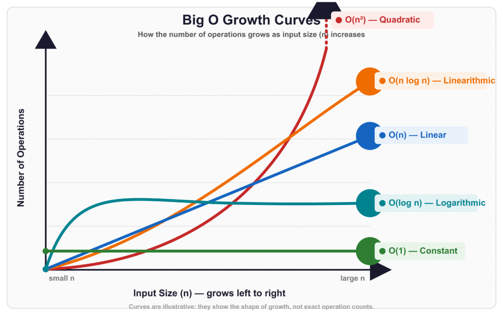
A useful way to think about their growth is:
O(1) → O(log n) → O(n) → O(n log n) → O(n²)
Generally, as you move toward the right, the algorithm becomes less scalable for very large inputs.
But remember: Big O is about growth, not a stopwatch. For small inputs, an algorithm with a theoretically worse complexity can sometimes be faster because of constants, implementation details, or overhead.
A Simple Example to Remember Everything
Imagine you have a list of students.
O(1)
You want to find the student at a specific position.
student = students[5]
You directly access the position.
O(1)
O(log n)
You search a sorted list by repeatedly cutting the search area in half.
O(log n)
O(n)
You check every student one by one.
for student in students:
print(student)
O(n)
O(n log n)
You use an efficient divide-and-conquer sorting algorithm such as Merge Sort.
O(n log n)
O(n²)
You compare every student with every other student.
for student1 in students:
for student2 in students:
print(student1, student2)
O(n²)
The Most Important Thing to Understand
Don’t just memorize these five Big O values.
Try to understand how the work grows.
If you remember that, the notation becomes much easier.
Think of it this way:
O(1) → “I can do it directly.”
O(log n) → “I can keep cutting the problem down.”
O(n) → “I need to look at each item.”
O(n log n) → “I divide the problem and process the pieces efficiently.”
O(n²) → “For each item, I may have to look at many other items.”
Once you can recognize these patterns in Python code, calculating Big O becomes much easier.
Quick Complexity Reference
| Notation | Name | Example |
|---|---|---|
| O(1) | Constant | Accessing an item by index |
| O(log n) | Logarithmic | Binary search |
| O(n) | Linear | Looping through a list once |
| O(n log n) | Linearithmic | Merge sort, Python’s sorted() |
| O(n²) | Quadratic | Nested loops over the same input |
How to Calculate Time Complexity
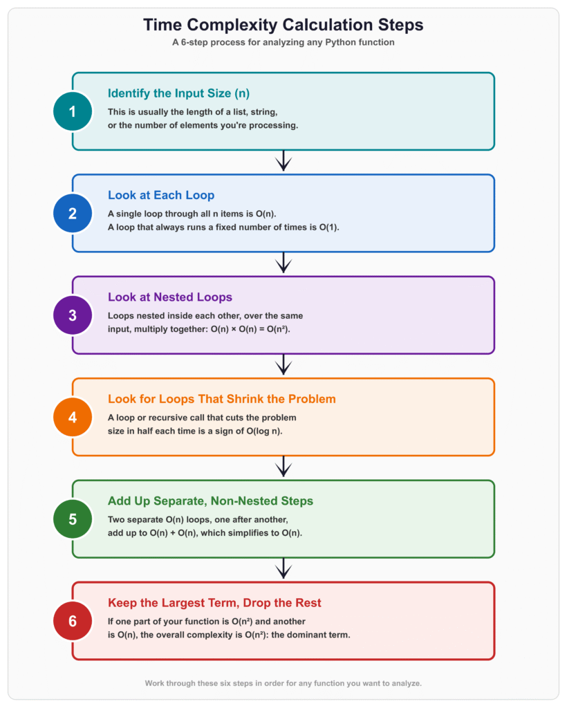
You do not need a formal proof to calculate Big O for most code. You need a simple, repeatable process. Here is one that works for the majority of everyday functions.
Step 1: Identify the input size, n. This is usually the length of a list, string, or the number of elements you are processing.
Step 2: Look at each loop. A single loop that runs through all n items is O(n). A loop that runs a fixed number of times, like exactly 5 times regardless of input, does not depend on n, so it counts as O(1).
Step 3: Look at nested loops. If a loop sits inside another loop, and both depend on the same input size, multiply their complexities. Two nested loops over the same n items give O(n) times O(n), which is O(n²).
Step 4: Look at loops that shrink the problem. If a loop or recursive call cuts the problem size in half (or by some fraction) each time, that is a sign of O(log n).
Step 5: Add up separate, non-nested steps. If your function does one O(n) loop, then a separate O(n) loop afterward (not nested), that is O(n) + O(n), which simplifies to O(n). Big O only cares about the fastest-growing term, so you drop constants and lower-order terms.
Step 6: Keep the largest term, and drop the rest. If a function does O(n²) work in one part and O(n) work in another, the overall complexity is O(n²), because that term dominates as n grows.
Let’s walk through a real example:
def process(items):
total = 0 # O(1)
for item in items: # O(n)
total += item
seen = set()
for item in items: # O(n), separate from the loop above
seen.add(item)
return total, seenTwo separate O(n) loops, one after another. That adds up to O(n) + O(n) = O(2n), and Big O drops the constant, giving you O(n) overall.
Now compare it to this:
def process_pairs(items):
pairs = []
for i in items: # O(n)
for j in items: # O(n), nested inside the first loop
pairs.append((i, j))
return pairsHere the second loop is nested inside the first, so you multiply: O(n) times O(n) = O(n²).
How to Calculate Space Complexity
Calculating space complexity uses the same mindset, but you track memory instead of steps. Ask yourself: as n grows, does the amount of extra memory this function uses grow too?
Step 1: Ignore the input itself. If a function receives a list as a parameter, that list already exists in memory before the function runs. Space complexity usually measures the additional memory the function creates.
Step 2: Look for new data structures. If the function creates a new list, set, or dictionary that grows with the input, that is O(n) space.
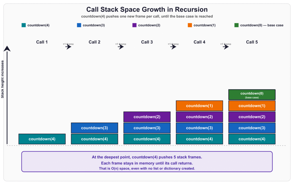
Step 3: Look at the call stack for recursion. Every recursive call adds a new frame to the call stack, and that frame stays in memory until the call returns. A recursive function that calls itself n times uses O(n) space, even if it never creates a single list or dictionary.
Here is a recursive example that shows this clearly:
def countdown(n):
if n <= 0:
return
countdown(n - 1)This function does not create any list or dictionary. It looks like it should use no extra memory. But each call to countdown stays on the call stack until the recursion below it finishes. Calling countdown(1000) creates 1,000 stacked function calls before any of them return.
It helps to break the total space down into parts:
- Recursive call stack: O(n), one frame for each active call
- Explicit data structures created: O(1), since no list, set, or dictionary is created
- Total auxiliary space: O(n), because the call stack dominates
Compare that to the earlier sum_of_list function. It loops instead of recursing, so it never builds up a call stack, and it uses O(1) space overall.
This is one of the most overlooked ideas in space complexity: recursion is not “free” just because you did not explicitly create a data structure. The call stack itself counts as memory.
Common Big O Mistakes
These mistakes show up constantly, even among developers who understand the concept in theory.
Mistake 1: Confusing “fast in testing” with “fast at scale.” Code that runs quickly on a list of 20 items can still be O(n²). Small inputs hide bad complexity. Always ask “what happens if this input were 100 times bigger?” instead of trusting a quick test run.
Mistake 2: Assuming every nested loop means O(n²). This is not always true. If the inner loop does not depend on the size of the outer loop’s input, and instead runs a fixed number of times, it does not multiply the way you’d expect.
def print_first_three(items):
for item in items: # O(n)
for i in range(3): # Always exactly 3 iterations, not O(n)
print(item, i)This is O(n), not O(n²), because the inner loop always runs exactly 3 times, regardless of n.
The safest way to check is to ask: “does the inner loop’s range depend on the input size, or is it fixed?” Sometimes the inner loop does depend on the input, but not in a way that repeats the full outer loop. For example:
def print_triangle(items):
for i in range(len(items)):
for j in range(i):
print(items[i], items[j])Here the inner loop’s range depends on i, so it is not a fixed number like the last example. But it is also not a full n iterations every time. The inner loop runs 0 times, then 1, then 2, and so on, up to n - 1. Added together, that totals roughly n² / 2 operations, which still simplifies to O(n²), since Big O drops constants. The lesson here is to actually trace through what each loop does, instead of assuming “nested loop always means O(n²)” or “nested loop never means O(n²).” Both assumptions can be wrong. Read the loop bounds.
Mistake 3: Forgetting that built-in operations have their own cost. It is easy to assume every line of code is O(1). But operations like in on a Python list, or inserting at the front of a list, are O(n) themselves, because Python has to check or shift every element.
def contains(items, target):
return target in items # O(n) on a list, not O(1)Checking membership in a set or dict, however, is typically O(1) on average, because of how hashing works. This single difference (list vs set for membership checks) is one of the most common causes of accidentally slow Python code.
Mistake 4: Ignoring space complexity entirely. Many developers only think about time. But an algorithm that is fast in time and terrible in memory can crash a program on large inputs just as easily as a slow one can time out.
Mistake 5: Treating Big O as an exact prediction of runtime. Big O tells you about growth rate, not literal seconds. Two O(n) functions can run at very different real speeds, because of constants, hardware, and implementation details. Big O tells you the shape of the curve, not the exact time on the clock.
Big O Examples in Python
A few more grounded, side-by-side examples, since seeing the pattern repeated in different situations helps it stick.
# O(1): Constant time
def get_last_item(items):
return items[-1]
# O(log n): Logarithmic time
def power_of_two_search(n):
count = 0
while n > 1:
n = n // 2
count += 1
return count
# O(n): Linear time
def find_max(items):
max_value = items[0]
for item in items:
if item > max_value:
max_value = item
return max_value
# O(n log n): Linearithmic time
def sorted_copy(items):
return sorted(items)
# O(n²): Quadratic time
def all_pairs_sum(items):
results = []
for i in items:
for j in items:
results.append(i + j)
return resultsReading through code like this, and asking “what is n here, and how does the work scale with it,” is the fastest way to build real intuition for Big O.
Big O Cheat Sheet
| Complexity | Intuition | Typical example |
|---|---|---|
| O(1) | Doesn’t grow with input | List indexing |
| O(log n) | Grows very slowly | Binary search |
| O(n) | Grows proportionally with input | Linear scan |
| O(n log n) | Slightly faster-growing than linear | Efficient sorting |
| O(n²) | Grows rapidly | Nested loops, pairwise comparisons |
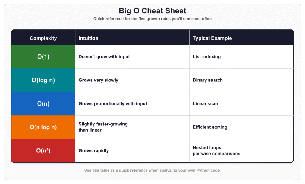
As a rule of thumb: O(1) and O(log n) tend to stay manageable even as input grows very large. O(n) and O(n log n) scale reasonably well for most real-world data sizes. O(n²) and worse are the ones to watch closely, since the actual runtime can grow rapidly once your input reaches the thousands or millions. This is about growth trend, not a guarantee about literal speed. A constant-time operation with heavy overhead can still be slower in practice than a linear one with very little overhead, especially on small inputs.
Big O Interview Questions for FAANG-Style DSA Interviews
If you’re preparing for DSA interviews at companies such as Google, Amazon, Meta, Apple, or Microsoft, you should be comfortable analyzing the time and space complexity of your Python code. Interviewers often care not only about getting the correct answer, but also about explaining how efficiently your solution scales.
Here are some important interview questions to practice.
1. What is Big O notation?
Answer:
Big O notation describes how an algorithm’s time or memory requirements grow as the input size n increases.
For example:
O(1)→ ConstantO(log n)→ LogarithmicO(n)→ LinearO(n log n)→ LinearithmicO(n²)→ Quadratic
Big O focuses on the growth rate, rather than the exact execution time.
2. What is the time complexity of this Python code?
numbers = [1, 2, 3, 4, 5]
for number in numbers:
print(number)
Answer:
The loop visits every element once.
If there are n elements, the loop runs n times.
Time Complexity: O(n)
Space Complexity: O(1) if we don’t count the input list itself.
3. What is the time complexity of nested loops?
numbers = [1, 2, 3, 4, 5]
for i in numbers:
for j in numbers:
print(i, j)
Answer:
The outer loop runs n times.
For every iteration of the outer loop, the inner loop also runs n times.
Therefore:
n × n = n²
Time Complexity: O(n²)
Space Complexity: O(1)
4. What is the time complexity of accessing an element by index in a Python list?
numbers = [10, 20, 30, 40, 50]
print(numbers[3])
Answer:
Python lists provide direct access by index.
We don’t need to search through the previous elements.
Time Complexity: O(1)
Space Complexity: O(1)
5. What is the time complexity of searching for a value in a Python list?
numbers = [10, 20, 30, 40, 50]
if 40 in numbers:
print("Found")
Answer:
Python may need to check each element until it finds the value.
In the worst case, it checks all n elements.
Time Complexity: O(n)
Space Complexity: O(1)
6. What is the time complexity of binary search?
Answer:
Binary search repeatedly divides the search space into half.
For example:
n → n/2 → n/4 → n/8 → ...
Because the search space is reduced by half at every step, the time complexity is:
O(log n)
Binary search requires the data to be appropriately sorted.
7. What is the difference between O(n) and O(log n)?
Answer:
With O(n), the algorithm may need to process every element.
With O(log n), the algorithm can eliminate a large portion of the input at each step.
For example:
Linear search → O(n)
Binary search → O(log n)
As n becomes very large, O(log n) grows much more slowly than O(n).
8. What is the time complexity of this code?
numbers = [1, 2, 3, 4, 5]
for i in range(len(numbers)):
for j in range(i + 1, len(numbers)):
print(numbers[i], numbers[j])
Answer:
There are two nested loops, and the number of iterations grows approximately with the square of n.
Therefore:
Time Complexity: O(n²)
Space Complexity: O(1)
The exact number of iterations is smaller than n², but Big O ignores constant factors and lower-order terms.
9. What is the time complexity of Python’s sort()?
numbers.sort()
Answer:
Python’s built-in list sorting uses Timsort.
Its worst-case time complexity is:
O(n log n)
Python’s official documentation provides the complexity details for built-in data structures and operations, making it a useful reference when analyzing Python code.
10. What is the difference between time complexity and space complexity?
Answer:
Time complexity describes how the amount of computational work grows as the input becomes larger.
Space complexity describes how the memory requirements grow.
For example:
def double_numbers(numbers):
result = []
for number in numbers:
result.append(number * 2)
return result
The function processes every element once.
Time Complexity: O(n)
But it also creates a new list containing n elements.
Auxiliary Space: O(n)
11. Can an algorithm have O(n) time and O(1) space?
Answer:
Yes.
For example:
def find_max(numbers):
maximum = numbers[0]
for number in numbers:
if number > maximum:
maximum = number
return maximum
We examine every element once:
Time: O(n)
But we only use a few variables regardless of the input size:
Auxiliary Space: O(1)
12. Which is better: O(n) or O(n²)?
Answer:
Generally, O(n) is better for large inputs because it grows much more slowly than O(n²).
For example, when n = 1,000:
O(n) → approximately 1,000 operations
O(n²) → approximately 1,000,000 operations
However, Big O isn’t a stopwatch. For very small inputs, constants and implementation details can make the practical performance different.
13. What is the time complexity of this code?
for i in range(n):
print(i)
for j in range(n):
print(j)
Answer:
The first loop runs n times.
The second loop also runs n times.
So the total work is:
n + n = 2n
We drop the constant 2.
Therefore:
Time Complexity: O(n)
This is an important interview concept: two consecutive O(n) loops are still O(n), not O(n²).
14. What is the time complexity of this code?
for i in range(n):
for j in range(n):
print(i, j)
for k in range(n):
print(k)
Answer:
The nested loops take:
O(n²)
The final loop takes:
O(n)
Together:
O(n² + n)
We keep the term that grows faster and drop the smaller term.
Therefore:
Time Complexity: O(n²)
15. Can you improve an O(n²) solution to O(n)?
Answer:
Sometimes, yes.
A common example is searching for duplicate values.
A brute-force approach might compare every element with every other element:
for i in range(len(numbers)):
for j in range(i + 1, len(numbers)):
if numbers[i] == numbers[j]:
return True
This takes:
O(n²) time.
We can often use a Python set to remember values we’ve already seen:
seen = set()
for number in numbers:
if number in seen:
return True
seen.add(number)
return False
The average-case time complexity becomes:
O(n)
But we now use additional memory:
Space Complexity: O(n)
This is a classic example of a time-space trade-off: we use more memory to reduce the amount of work.
Quick Interview Revision
Before an interview, make sure you can answer these without hesitation:
| Question | Answer |
|---|---|
| Array/list index access? | O(1) |
| Search in an unsorted list? | O(n) |
| Binary search? | O(log n) |
One loop through n elements? | O(n) |
| Two nested loops? | O(n²) |
| Efficient comparison-based sorting? | O(n log n) |
| Two separate O(n) loops? | O(n) |
| O(n²) + O(n)? | O(n²) |
Store n additional elements? | O(n) space |
| Use only a few extra variables? | O(1) space |
The interview habit you should develop
When you finish writing a solution, don’t stop at:
“My code works.”
Get into the habit of saying:
“The time complexity is O(n), because I traverse the input once. The auxiliary space is O(1), because I only use a constant number of extra variables.”
That one habit will make your DSA explanations much stronger in technical interviews.
Important: These are representative interview-style questions, not guaranteed questions from a particular company’s current interview pool. Exact questions vary by team, level, location, and interview. Current preparation sources consistently emphasize complexity analysis as a core DSA interview skill.
Big O Practice Problems
Now it’s time to test your understanding.
For each problem, try to answer these two questions:
- What is the time complexity?
- What is the space complexity?
Don’t look for the answer immediately. Try to analyze the code yourself first.
Problem 1 — Simple Loop
What is the time complexity?
numbers = [1, 2, 3, 4, 5]
for number in numbers:
print(number)
Your answer: O(?)
Problem 2 — Accessing an Element
What is the time complexity?
numbers = [10, 20, 30, 40, 50]
print(numbers[2])
Your answer: O(?)
Problem 3 — Searching a List
What is the worst-case time complexity?
numbers = [10, 20, 30, 40, 50]
target = 50
for number in numbers:
if number == target:
print("Found")
break
Your answer: O(?)
Problem 4 — Two Separate Loops
What is the time complexity?
numbers = [1, 2, 3, 4, 5]
for number in numbers:
print(number)
for number in numbers:
print(number * 2)
Your answer: O(?)
Hint: The loops are next to each other, not inside each other.
Problem 5 — Nested Loops
What is the time complexity?
numbers = [1, 2, 3, 4, 5]
for i in numbers:
for j in numbers:
print(i, j)
Your answer: O(?)
Problem 6 — Nested Loop with a Constant
What is the time complexity?
numbers = [1, 2, 3, 4, 5]
for number in numbers:
for i in range(10):
print(number, i)
Your answer: O(?)
Hint: range(10) always runs 10 times. It does not depend on n.
Problem 7 — Find the Maximum
What are the time and space complexities?
def find_max(numbers):
maximum = numbers[0]
for number in numbers:
if number > maximum:
maximum = number
return maximum
Your answer:
Time: O(?)
Space: O(?)
Problem 8 — Creating a New List
What are the time and space complexities?
def double_numbers(numbers):
result = []
for number in numbers:
result.append(number * 2)
return result
Your answer:
Time: O(?)
Space: O(?)
Problem 9 — Using a Set
What is the average-case time complexity?
def has_duplicate(numbers):
seen = set()
for number in numbers:
if number in seen:
return True
seen.add(number)
return False
Your answer:
Time: O(?)
Space: O(?)
Think carefully: Why does using a set make this solution different from comparing every pair?
Problem 10 — Binary Search
Consider the idea behind binary search:
def binary_search(numbers, target):
    left = 0
    right = len(numbers) - 1

    while left <= right:
        middle = (left + right) // 2

        if numbers[middle] == target:
            return middle
        elif numbers[middle] < target:
            left = middle + 1
        else:
            right = middle - 1

    return -1
What is the time complexity?
What is the space complexity of this iterative implementation?
Your answer:
Time: O(?)
Space: O(?)
Challenge Problems
If the first 10 problems feel comfortable, try these.
Problem 11 — What’s the Complexity?
def example(numbers):
for i in range(len(numbers)):
for j in range(i + 1, len(numbers)):
print(numbers[i], numbers[j])
Your answer: O(?)
Problem 12 — Three Loops
def example(numbers):
for number in numbers:
print(number)
for number in numbers:
print(number)
for number in numbers:
print(number)
Your answer: O(?)
Problem 13 — Nested + Separate Loop
def example(numbers):
for i in numbers:
for j in numbers:
print(i, j)
for number in numbers:
print(number)
Your answer: O(?)
Problem 14 — Which One Is Better?
You have two solutions to the same problem.
Solution A:
def find_duplicate(numbers):
for i in range(len(numbers)):
    for j in range(i + 1, len(numbers)):
        if numbers[i] == numbers[j]:
            return True
return False
Solution B:
def find_duplicate(numbers):
seen = set()

for number in numbers:
    if number in seen:
        return True

    seen.add(number)

return False
Answer these questions:
- What is the time complexity of Solution A?
- What is the time complexity of Solution B?
- What is the space complexity of Solution A?
- What is the space complexity of Solution B?
- Which solution would you prefer for a very large input?
- What trade-off does Solution B make?
Answers
Try solving all the problems yourself before reading this section.
Problem 1
Time: O(n)
The loop processes every element once.
Space: O(1) if we don’t count the input list.
Problem 2
Time: O(1)
Python can access a list element directly by its index.
Space: O(1)
Problem 3
Time: O(n)
In the worst case, the target can be at the end of the list, so we may need to check every element.
Space: O(1)
Problem 4
Time: O(n)
The first loop is O(n).
The second loop is also O(n).
So:
O(n) + O(n) = O(2n)
We drop the constant:
O(n)
Problem 5
Time: O(n²)
The outer loop runs n times, and the inner loop runs n times for each outer iteration.
n × n = n²
Problem 6
Time: O(n)
The inner loop always runs 10 times.
So the total work is:
n × 10 = 10n
We drop the constant 10.
O(n)
Problem 7
Time: O(n)
We examine every element once.
Space: O(1)
Only a few variables are used.
Problem 8
Time: O(n)
Every input element is processed once.
Space: O(n)
The new result list contains n elements.
Problem 9
Average Time: O(n)
Set lookup and insertion are O(1) on average, so we process n elements.
Space: O(n)
The seen set can contain up to n elements.
Problem 10
Time: O(log n)
The search space is cut roughly in half on every iteration.
Space: O(1)
This is an iterative implementation, so it doesn’t create a recursive call stack.
Problem 11
Time: O(n²)
Although the inner loop doesn’t always run exactly n times, the total number of comparisons grows quadratically.
O(n²)
Problem 12
Time: O(n)
The three loops are sequential:
O(n) + O(n) + O(n) = O(3n)
Drop the constant:
O(n)
Problem 13
Time: O(n²)
The nested loops require O(n²).
The additional loop requires O(n).
So:
O(n²) + O(n) = O(n²)
We keep the term that grows faster.
Problem 14
Solution A:
Time: O(n²)
Space: O(1)
Solution B:
Average time: O(n)
Space: O(n)
For a very large input, Solution B is generally preferable because it reduces the running time significantly by using extra memory.
This is a classic example of a:
Time-space trade-off
Interview Tip
When an interviewer gives you a piece of code and asks for its Big O, don’t guess immediately.
Follow these steps:
Step 1: Identify what n represents.
Step 2: Count how many times each loop runs.
Step 3: Check whether loops are nested or sequential.
Step 4: Look for operations such as searching, sorting, slicing, or creating new data structures.
Step 5: Simplify the final expression.
For example:
O(n² + n + 10)
becomes:
O(n²)
because n² grows faster than n and the constant 10.
The goal isn’t just to memorize Big O values. You should be able to look at Python code and explain why it has that complexity.
Frequently Asked Questions
Is Big O the same as runtime in seconds?
No. Big O describes how work grows as input grows, not the literal number of seconds a program takes. Two O(n) functions can run at different real speeds depending on hardware and implementation details.
What is the difference between Big O, Big Omega, and Big Theta?
Big O describes an asymptotic upper bound on growth. Big Omega describes an asymptotic lower bound on growth. Big Theta describes a tight bound, where the upper and lower bounds match. None of the three is inherently tied to “worst case” or “best case.” In everyday conversation, though, people usually pair Big O with worst-case behavior, because that is the number most useful for planning around. Big O is the one used most often in everyday discussion and interviews.
Is O(1) always faster than O(n)?
Not necessarily, for every input size. O(1) has a better asymptotic growth rate than O(n), meaning it scales better as input grows toward infinity. But actual runtime also depends on constants, implementation details, and hardware, not growth rate alone. A constant-time operation with a lot of overhead can still be slower than a linear operation on a small input. Big O tells you which one wins as
ngets large, not which one is faster for every single input size.Do I need to calculate Big O for every function I write?
Not every function, but you should build the habit of thinking through it for any code that processes lists, strings, or other growing data, especially in loops or recursive calls.
Why do interviewers care so much about Big O?
Because it shows whether you understand the actual behavior of your solution, not just whether it produces the right output on a small test case. It is one of the fastest ways to tell if a candidate can reason about code, not just write it.
Can space complexity matter more than time complexity?
Yes, in some cases. An algorithm that runs fast but uses too much memory can crash on large inputs before a slower, more memory-efficient algorithm would even struggle.
Big O vs Best, Average, and Worst Case
Before wrapping up, it is worth untangling one more idea, since it trips up a lot of beginners: Big O is not the same thing as “worst case,” even though the two get used together so often that people start to think they are one and the same.
- Best case: how the algorithm behaves on the most favorable input. Searching a list where the target happens to be the first item is a best case.
- Worst case: how the algorithm behaves on the least favorable input. Searching a list where the target is the last item, or is not there at all, is a worst case.
- Average case: the expected behavior across a typical range of inputs, not just the extremes.
- Big O: a notation for describing how growth scales. It can be used to describe the best case, the worst case, or the average case. It is not, by itself, a synonym for “worst case.”
In everyday use, when someone says “this function is O(n),” they usually mean its worst-case behavior is O(n), because worst case is the most useful number to plan around. That convention is common enough that it rarely causes confusion in practice. But it helps to know that this is a convention, not a strict rule, since some algorithms have very different best-case and worst-case complexities. Binary search, for example, has a best case of O(1) (the target happens to be the exact middle element) and a worst case of O(log n). The next article in this series covers this distinction in more depth.
Conclusion
Big O notation gives you a way to reason about your code before it becomes a problem in production. It is not about counting exact operations. It is about understanding the shape of growth: does your code stay flat, grow steadily, or explode as input size increases?
The habit worth building from here is simple: whenever you write a loop or a recursive function, pause and ask what n is, and how the work scales with it. That single habit will make you a noticeably stronger Python developer and a much stronger interview candidate.
If you want to see how this fits into the bigger picture, the complete DSA with Python guide lays out the full learning path from here.
From here, the next article in this series looks at best-case, average-case, and worst-case time complexity, and why the exact same algorithm can behave very differently depending on which input it happens to receive.
External Resources
- Python Documentation — Time Complexity of Built-in Types
A very useful reference when you start analyzing actual Python code. It lists the complexity of operations such as list access,append(), searching within, sorting, slicing, and more.
Python Time Complexity Documentation - MIT OpenCourseWare — Understanding Program Efficiency
This is a university-level resource from MIT that introduces algorithmic complexity, Big O notation, and different complexity classes. It is particularly relevant because the course itself teaches programming in Python.
MIT OpenCourseWare: Understanding Program Efficiency







Leave a Reply