

How to Analyze the Time and Space Complexity of an Algorithm
Time and Space Complexity:
This article is part of the Data Structures & Algorithms with Python roadmap. If you haven’t read the recursion in Python guide yet, start there. This article builds on it directly.
In Simple Terms
To find the time complexity of an algorithm, count how many times its operations run as the input grows. To find the space complexity, count how much extra memory it uses as the input grows. You don’t need to run the code to know this. You just need to read it carefully and ask: “What happens if the input gets bigger?”
Why This Skill Matters
You already know what Big O means. You know the difference between best, average, and worst case. You even know how to trace a recursive function and watch its call stack grow.
But here’s the part that trips people up. Knowing what O(n) means is not the same as looking at a random piece of code and knowing that it is O(n).
That second skill is the one interviewers actually test. They rarely ask “what is Big O?” They hand you a function and ask, “What’s the time complexity of this?” Then they wait.
This guide gives you a repeatable process for answering that question. Not a trick. Not a shortcut. A process you can run on almost any piece of Python code, step by step, until the answer falls out.
Start With the Input Size
Before you count a single operation, answer one question: what is “n” here?
This sounds obvious, but it’s the step people skip, and skipping it causes most of the confusion that follows.
Think of it like measuring a room before buying carpet. You wouldn’t start cutting carpet before you know the room’s dimensions. In the same way, you shouldn’t start counting operations before you know what’s actually growing.
Sometimes n is easy to spot. It’s the length of a list, or the number of items in a dictionary. Other times it’s less obvious.
- If the input is a string, n is usually the number of characters.
- If the input is a matrix, n might be the number of rows, the number of columns, or both.
- If the input is a number, like
factorial(n), n is the number itself, not the number of digits in it. - If a function takes two different collections, you might have two separate variables, n and m, instead of one.
Here’s a small example with two inputs:
def has_common_item(list_a, list_b):
    for a in list_a:
        for b in list_b:
            if a == b:
                return True
return FalseThere isn’t one “n” here. There’s the length of list_a and the length of list_b. Calling them both n would hide what’s actually happening. The honest way to describe this function’s complexity uses two variables: n for list_a and m for list_b.
Naming your input size correctly, before you count anything, keeps the rest of the analysis from going wrong.
Count the Operations
Once you know what n is, the next step is simple to say and takes practice to do well: count how many basic operations the code performs, in terms of n.
A “basic operation” is something that takes roughly constant time on its own. A comparison. An addition. A variable assignment. Reading a value from a list by index. None of these get slower as the input grows, on their own.
Take this function:
def get_first_and_last(items):
    first = items[0]
    last = items[-1]
return first, lastNo matter how long items is, this function does the same fixed amount of work. Two lookups, one return. Whether the list has 5 items or 5 million, the work doesn’t change. That’s O(1), constant time.
Compare that to this one:
def contains_value(items, target):
    for item in items:
        if item == target:
            return True
return FalseHere, the number of comparisons depends directly on how many items are in the list. In the worst case, the target isn’t there at all, and the loop checks every single item. That worst-case count grows in a straight line with n. That’s O(n), linear time.
The pattern to notice: constant-time code doesn’t touch every element. Linear-time code performs an amount of work that grows proportionally with the input size. Once you can tell those two apart on sight, the rest of this guide is about combining that same idea into more complex shapes.
One more thing worth knowing early: complexity depends on the data structure as well as the operation. Indexing a Python list with items[0] is O(1), while checking whether a value exists in that same list with in is O(n). The operation name alone doesn’t tell you the cost. The data structure behind it matters just as much.
Analyze Loops
A single loop over a collection is the most common shape you’ll analyze, so it’s worth having a clear rule for it.
Rule: A loop that runs once for every element in a collection of size n is O(n), as long as the work inside the loop is constant.
def print_all(items):
    for item in items:
print(item) # constant work per iterationn items, constant work each. Total work: O(n).
But loops don’t always run n times. Watch what happens when the loop’s step size changes:
def print_every_other(items):
    for i in range(0, len(items), 2):
print(items[i])This loop still depends on n, but it only runs about n / 2 times. In Big O, constants like that get dropped, because Big O describes growth rate, not an exact count. n / 2 still grows in a straight line as n grows, so this is still O(n). The constant factor doesn’t change the shape of the growth.
Now look at a loop that shrinks by a different pattern:
def halving_loop(n):
    count = 0
    while n > 1:
        n = n // 2
        count += 1
return countInstead of counting down by 1 each time, this loop cuts n in half every iteration. That changes the shape of the growth completely. If n doubles, this loop only needs one extra iteration, not twice as many. That “cut in half every step” pattern is the signature of O(log n), logarithmic time. You’ll see this exact shape again once you get to binary search later in this series.
Here’s a quick way to sanity check yourself: don’t ask what the loop does first. Ask how many times it runs as n grows. If it runs n times, it’s linear. If it runs log(n) times, it’s logarithmic. If it runs a fixed number of times no matter what n is, it’s constant.
Analyze Nested Loops
Nested loops are where a lot of people start guessing instead of counting. Here’s the rule that removes the guesswork.
Rule: When one loop sits inside another, multiply their individual costs together.
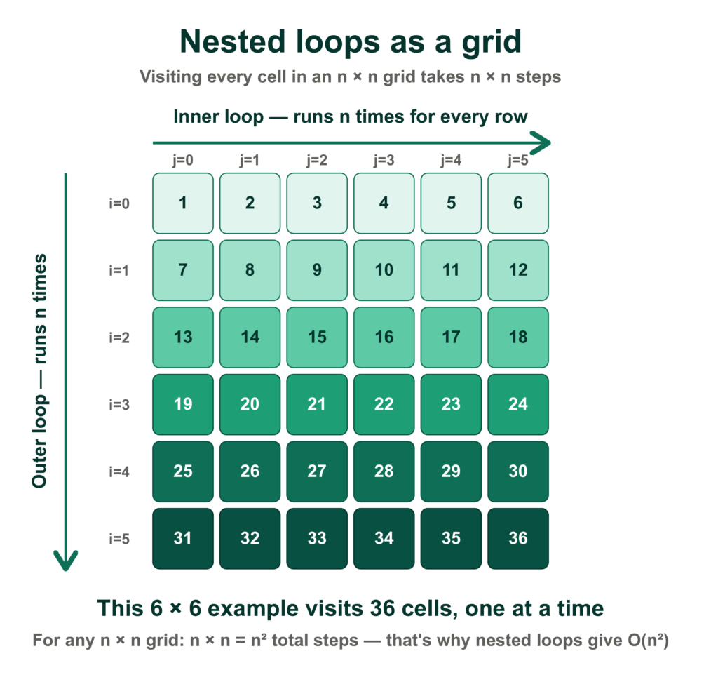
Picture it like a grid. If you visit every cell in a 5×5 grid, you visit 25 cells, not 10. You’re not adding the rows and columns together. You’re covering every combination of row and column.
def print_all_pairs(items):
    for a in items:
        for b in items:
print(a, b)The outer loop runs n times. For every single one of those n runs, the inner loop also runs n times. That gives you n × n total iterations, which is n². This function is O(n²), quadratic time.
Nested loops don’t always cover the same range, though. Look at this one:
def print_upper_triangle(items):
    for i in range(len(items)):
        for j in range(i, len(items)):
print(items[i], items[j])The inner loop’s range shrinks a little each time the outer loop advances. On the first pass, the inner loop runs n times. On the second pass, it runs n – 1 times. And so on, down to 1.
Add all of those up: n + (n – 1) + (n – 2) + … + 1. That sum works out to roughly n² / 2. The constant factor (the “/2”) gets dropped in Big O notation, but the shape is still quadratic. This function is O(n²), just like the first one, even though it does noticeably less actual work.
That last point matters: two pieces of code can have the same Big O and still run at very different speeds in practice. Big O tells you the growth shape, not the exact runtime. Don’t confuse the two.
What about three nested loops, all running over the same input? Follow the same multiplication rule: n × n × n = n³. Every extra layer of nesting over the same input size multiplies in another factor of n.
Analyze Conditionals
Conditionals (if, elif, else) don’t multiply your operation count the way loops do. Instead, they create branches, and you need to think about which branch matters for the case you’re analyzing.
def check_value(items, target):
    if len(items) == 0:
        return False          # O(1) branch
    for item in items:
        if item == target:
            return True
return FalseThere are two possible paths here. The empty-list path does a constant amount of work. The loop path does up to n comparisons. Since Big O worst-case analysis cares about the most expensive thing that can happen, you take the more expensive branch. The loop dominates, so the overall complexity is O(n).
A conditional inside a loop is a different situation, and it’s one that confuses people:
def count_even_numbers(numbers):
    count = 0
    for num in numbers:
        if num % 2 == 0:
            count += 1
return countHere, the if doesn’t create a separate path with a different cost. It’s just a constant-time check that runs on every iteration, whether the condition is true or false. The loop still runs n times either way. This function is O(n), the same as a loop with no conditional at all.
The rule to hold onto: a conditional that runs inside a loop, doing constant work either way, doesn’t change the loop’s complexity. A conditional that causes the function to do a completely different, more expensive amount of work in one branch is the one you need to account for separately, and you generally count the most expensive branch when you’re analyzing the worst case.
Analyze Recursion
A recursive function’s time complexity depends on how many calls it makes and how much work each call performs on its own. For branching recursion, where a single call can trigger more than one further call, you also need to account for how those calls grow into a recursion tree, not just multiply a flat call count by a flat work-per-call number.
Here’s that same idea applied as a repeatable process:
- How many times does the function call itself, and how does that branch (once per call, or more than once)?
- How much work does each individual call do on its own, ignoring the recursive call itself?
- For single-branch recursion, multiply calls by work-per-call for time. For branching recursion, work out how the recursion tree grows instead. Either way, look at the maximum stack depth for space.
Take this function, which finds the largest number in a list recursively:
def find_max(items, index=0, current_max=float('-inf')):
    if index == len(items):
        return current_max
    current_max = max(current_max, items[index])
return find_max(items, index + 1, current_max)One call per level, from index 0 up to len(items). Each call does one comparison, which is constant work. That’s n calls, times constant work per call: O(n) time. The call stack goes n levels deep before it starts returning, so the space complexity is also O(n).
Now compare it to naive recursive Fibonacci, which you saw in the previous article. Each call spawns two more calls instead of one. That branching causes the number of calls to grow exponentially, giving the usual naive implementation an O(2^n) time bound. (A tighter bound exists, Θ(φⁿ), where φ is the golden ratio, but O(2^n) is the standard, and perfectly acceptable, way to describe it at this stage.) The lesson to keep: it’s the shape of the recursion tree, driven by how many calls each call triggers, that determines the time cost, and the deepest single path through those calls that determines the space cost.
Analyze Multiple Parts of an Algorithm
Real functions are rarely just one loop. They’re usually a sequence of steps, sometimes followed by a nested structure, sometimes followed by another separate loop. Here’s how to combine them correctly.
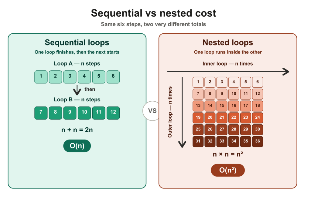
Rule for sequential steps: add their costs together, then keep only the largest term.
def process(items):
    for item in items:            # O(n)
        print(item)

    for i in range(len(items)):   # O(n^2)
        for j in range(len(items)):
print(items[i], items[j])The first loop costs O(n). The second, nested loop costs O(n²). Added together, that’s O(n) + O(n²). As n grows large, the n² term grows so much faster that the n term becomes irrelevant by comparison. Big O only cares about that dominant term, so the whole function is O(n²).
Think of it like planning a road trip that has a five-minute stop for coffee and a four-hour drive. You don’t describe the trip as “four hours and five minutes.” You just say it’s a four-hour trip. The small part gets absorbed into the big part.
Rule for one part feeding into another: this is different from two separate steps. Watch this one closely, because it’s a common mistake:
def has_duplicate_pairs(items):
    seen_pairs = set()
    for i in range(len(items)):          # runs n times
        for j in range(len(items)):      # runs n times, for each i
            pair = (items[i], items[j])
            if pair in seen_pairs:
                return True
            seen_pairs.add(pair)
return FalseThis isn’t “a loop, then another loop.” The inner loop is nested inside the outer one, so their costs multiply, not add: n × n = O(n²). In the worst case, when no matching pair is found until the loops finish, this is O(n²). That’s the case Big O worst-case analysis describes; an early return can end the function sooner on some inputs, but the worst-case bound is still what you report unless you’re specifically asked for best or average case.
It’s also easy to misread nested structure as sequential structure if you’re skimming instead of tracing carefully, so always check: is the second loop inside the first, or does it come after the first has already finished?
Calculate Space Complexity
Time complexity asks “how many operations.” Space complexity asks “how much extra memory.” People forget to check this one far more often than they forget to check time.
The key phrase is “extra memory.” The usual convention, and the one interviewers mean when they ask for auxiliary space, is that you don’t count the input itself, since it already exists before your function runs. You count what your function adds on top of that.
Constant space looks like this:
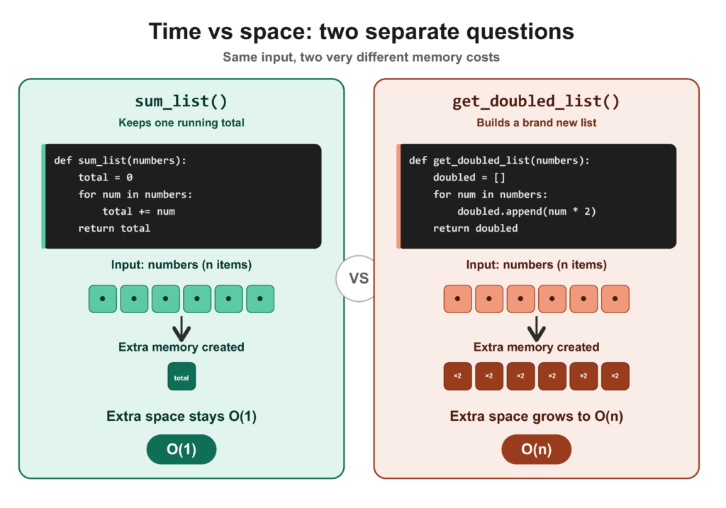
def sum_list(numbers):
    total = 0
    for num in numbers:
        total += num
return totalNo matter how long numbers is, this function only ever holds one extra variable, total. The input isn’t being copied or expanded anywhere. This is O(1) auxiliary space, even though it’s O(n) time. Time and space complexity are answers to two different questions, and they don’t have to match.
Now compare it to this version:
def get_doubled_list(numbers):
    doubled = []
    for num in numbers:
        doubled.append(num * 2)
return doubledThis function builds a brand new list that grows alongside the input. If numbers has n items, doubled ends up with n items too. That’s O(n) extra space, on top of whatever the original list was already using. This is also what “in-place” means when you see it in an algorithm description: an in-place algorithm modifies the existing input directly instead of building a new structure, which is why in-place algorithms are often described as O(1) space, regardless of how much time they take.
Recursion adds a space cost you can’t see just by reading the loop count, because the cost lives in the call stack, not in a variable you wrote yourself. You already saw this in the recursion article: a recursive function that goes n levels deep uses O(n) space for its call stack, even if it never creates a single list or dictionary of its own.
Here’s a quick way to check yourself: ask whether the function creates any new data structure whose size depends on the input (a new list, a new dictionary, a new set), and separately ask how deep any recursive calls go. Add those together, and you have your auxiliary space complexity.
Worked Python Examples
Let’s put the whole process together on three complete functions. For each one, walk through: input size, operation count, and space.
Example 1: Checking for duplicates, the slow way
def has_duplicate_slow(items):
    for i in range(len(items)):
        for j in range(len(items)):
            if i != j and items[i] == items[j]:
                return True
return False- Input size: n, the length of
items. - Loops: nested, both running roughly n times. That multiplies to O(n²) time in the worst case.
- Space: no new data structure grows with the input, just a couple of loop variables. O(1) space.
Example 2: Checking for duplicates, the fast way
def has_duplicate_fast(items):
    seen = set()
    for item in items:
        if item in seen:
            return True
        seen.add(item)
return False- Input size: still n.
- Loop: a single pass over the items, so O(n) iterations.
- Inside the loop: checking membership in a set and adding to a set are both O(1) on average, since Python sets are hash-based.
- Time: O(n) iterations × O(1) work each = O(n) time.
- Space: the
seenset can grow to hold up to n items, so O(n) space.
This pair is worth sitting with. The first version uses no extra memory but does far more work. The second version uses more memory but finishes much faster. That trade-off, spending memory to save time, shows up constantly in real code, and you’ll see it again soon under the name “hashing patterns” later in this series.
Example 3: A function with two separate inputs
def shared_items(list_a, list_b):
    result = []
    for a in list_a:
        for b in list_b:
            if a == b:
                result.append(a)
                break
return result- Input size: two separate variables. n for
list_a, m forlist_b. - Loops: nested, one over each list. That gives O(n × m) time, not O(n²), because the two loops don’t run over the same collection. The
breakends the inner loop early once a match is found, but that doesn’t change the worst-case bound, since in the worst case (no early matches) the inner loop still runs close to its full length for many values ofa. - Space:
resultcan contain at most the number of distinct shared values, so its worst-case size is O(min(n, m)). The extra space is O(min(n, m)).
This example is here specifically to break the habit of writing n² automatically whenever you see two nested loops. Multiply the actual sizes involved. They’re only the same variable when both loops run over the same collection.
There’s a small trap hiding in a version of this function you might write instinctively: checking a not in result before appending, to avoid duplicates.
def shared_items_with_membership_check(list_a, list_b):
    result = []
    for a in list_a:
        for b in list_b:
            if a == b and a not in result:
                result.append(a)
return resulta not in result looks like a constant-time check, but result is a list, and checking membership in a list is O(k), where k is the list’s current size. That membership check is quietly hiding inside your nested loops. It pushes the worst-case time up to O(n × m × min(n, m)), not O(n × m). If you want the O(n × m) version, either drop the membership check and dedupe afterward, or swap result for a set while building it, since set membership is O(1) on average.
The broader lesson: an operation’s cost depends on the data structure it’s running against, not just on how the code reads. in on a set and in on a list look identical on the page and cost completely different amounts.
How to Recognize Common Complexity Patterns
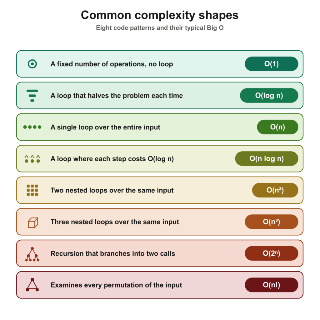
A few shapes come up over and over, once you start looking for them. This table is a summary of the patterns you’ve just walked through, not a new set of things to memorize separately.
| Code shape | Typical complexity |
|---|---|
| A fixed number of operations, no loop over the input | O(1) |
| A loop that cuts the problem in half each time | O(log n) |
| A single loop over the input | O(n) |
| A single loop where each step does O(log n) work | O(n log n) |
| Two nested loops over the same input | O(n²) |
| Three nested loops over the same input | O(n³) |
| A recursive function that branches into two calls per call | O(2^n) |
| Generates or examines every permutation of the input | O(n!) |
You don’t need to memorize this table word for word. What’s worth remembering is the shape each pattern comes from: halving means logarithmic, one full pass means linear, nested passes over the same data mean polynomial, and branching recursive calls mean exponential.
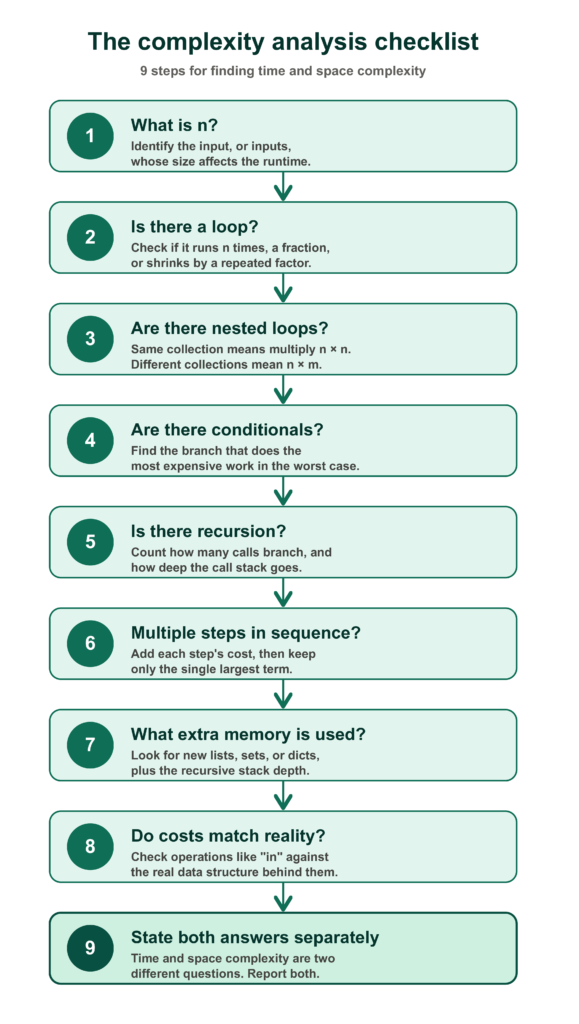
Complexity Analysis Checklist
Run through these questions, in order, any time you need to find the complexity of a piece of code.
- What is n? Identify the input, or inputs, whose size actually affects the runtime.
- Is there a loop? If so, does it run n times, a fraction of n times, or does it shrink by a repeated factor (like halving)?
- Are there nested loops? If so, do they run over the same collection (n × n) or different collections (n × m)? Multiply their costs.
- Are there conditionals? Do they just add a constant check inside a loop, or do they create a genuinely more expensive separate path?
- Is there recursion? How many calls happen, and how do they branch? How deep does the call stack go at its tallest point?
- Are there multiple steps in sequence? Add their individual costs, then keep only the largest term.
- What extra memory does the function create? Look for new lists, dictionaries, sets, or strings that grow with the input, and add the recursive call stack depth if there is one.
- Does every operation cost what it looks like it costs? Check
in, membership tests, and lookups against the actual data structure they run on, not just against how the code reads. - State both answers separately. Time complexity and space complexity are two different questions. Don’t assume one tells you the other.
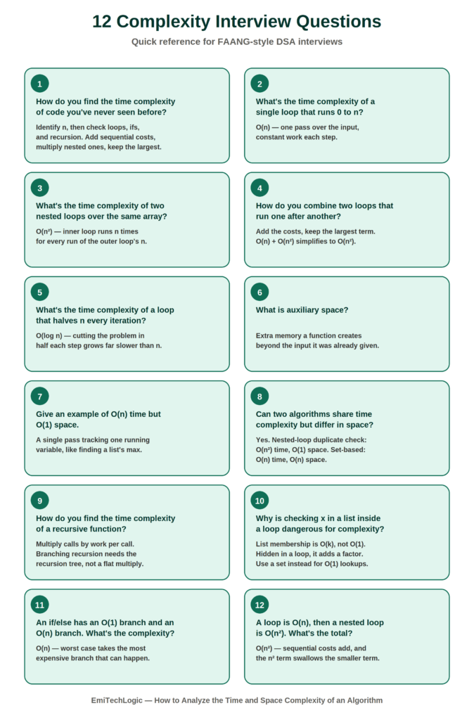
FAANG-Style DSA Interview Questions
Save this poster so you have all 12 answers on one page for quick review before an interview.
1. How do you find the time complexity of a piece of code you’ve never seen before?
Identify n first, then walk the code top to bottom asking “how many times does this run as n grows?” for every loop, conditional, and recursive call. Add costs that happen in sequence, multiply costs that are nested inside each other, and report only the largest term.
Take this function:
def process(items):
    total = sum(items)          # O(n)
    for i in range(len(items)):
        for j in range(len(items)):
print(items[i], items[j]) # O(n^2)The sum is O(n), the nested loop is O(n²). They run in sequence, so you add them: O(n) + O(n²). Since n² dominates for large n, the answer is O(n²). Saying that reasoning out loud is exactly what most interviewers are listening for, not just the final answer.
2. What is the time complexity of a single loop that runs from 0 to n?
O(n). Each iteration does constant work, and the loop runs once per element, so total work scales in a straight line with input size.
for x in items: print(x) is O(n). But watch for a trap: for x in items: print(x); print(x); print(x) is still O(n) — three constant-time prints per iteration is still constant work per iteration, just with a bigger constant. Don’t let extra lines inside a loop trick you into raising the complexity class.
3. What is the time complexity of two nested loops over the same array?
O(n²), because the inner loop runs n times for every one of the outer loop’s n runs, giving n × n total iterations.
A brute-force duplicate check (for i: for j: if items[i]==items[j]) is the classic O(n²) case. In an interview, immediately follow up with the optimization: you can bring this to O(n) time by trading it for O(n) space with a set. Naming that trade-off unprompted is what separates a pass from a strong pass.
4. If two loops run one after another instead of being nested, how do you combine their costs?
Add them, then drop everything except the largest term. O(n) + O(n²) simplifies to O(n²), because for large n the n² term makes the n term negligible.
Don’t just cite the rule, apply it live. If someone hands you a function with a linear pass followed by a nested loop, say the sum out loud (O(n) + O(n²)), then explicitly cross out the smaller term before giving the final answer. That visible step proves you understand why the rule works, not just that it exists.
5. What is the time complexity of a loop that cuts n in half every iteration?
O(log n). Each step removes a fixed fraction of what’s left rather than a fixed count, so the number of iterations barely grows even as n grows a lot.
while n > 1: n = n // 2 — if n starts at 1,000,000, this loop runs about 20 times, not a million. That’s the practical payoff of recognizing O(log n): it tells you an algorithm will still feel fast even on huge inputs, which is exactly why binary search scales so well.
6. What is auxiliary space, and why don’t we count the input itself?
Auxiliary space is the extra memory a function allocates beyond what was handed to it. The input already exists in memory before the function is called, so counting it would double-count memory the function didn’t create.
def total(nums): return sum(nums) uses O(1) auxiliary space. It doesn’t matter that nums might be a million items, because the function itself allocates nothing beyond one running number. Say “auxiliary space” instead of just “space” in an interview. It signals you know the distinction and don’t need it clarified.
7. Can you give an example of an algorithm with O(n) time complexity but O(1) space complexity?
Any single pass over the input that only tracks a constant number of variables.
def find_max(nums):
    best = nums[0]
    for n in nums:
        if n > best:
            best = n
return bestOne pass gives O(n) time, and one variable that never grows gives O(1) space. This is a good one to have ready, because it’s the cleanest possible demonstration that time and space are answering different questions.
8. Can two algorithms have the same time complexity but different space complexity?
Yes, and this is the point where a lot of candidates lose points by assuming one number tells you the other.
Checking for duplicates with a nested loop is O(n²) time, O(1) space. Checking with a set is O(n) time, O(n) space. Say both numbers for both approaches, every time you compare two solutions in an interview, never just the time complexity. That habit alone makes your answers sound senior.
9. How do you find the time complexity of a recursive function?
Multiply how many calls happen by how much work each call does on its own. For single-branch recursion, one call per call, that’s straightforward multiplication. For branching recursion, you have to reason about how the recursion tree grows, since the call count itself is what’s expanding.
factorial(n) makes n calls, each doing one multiplication, giving O(n). Naive fibonacci(n) makes two calls per call, so the call count roughly doubles each level down, giving O(2^n). If you’re ever unsure, sketch the first three levels of the recursion tree on the whiteboard. It makes the branching factor visually obvious instead of something you have to guess at.
10. Why is checking x in some_list inside a loop dangerous for complexity?
List membership is O(k), where k is the list’s current length, not O(1). Hidden inside another loop, that turns what looks like O(n) into something much worse.
seen = []
for x in items:
    if x not in seen:      # O(k), a hidden cost
seen.append(x)This is O(n²) in the worst case, not O(n), because of the membership check. Swap seen for a set() and the logic stays the same, but membership becomes O(1) instead of O(k), so the whole function becomes a genuine O(n). This is one of the highest-value things to catch out loud in an interview, because it shows you read code for real cost, not just surface shape.
11. If a function has an if/else where one branch is O(1) and the other is O(n), what is its overall time complexity?
O(n). Worst-case analysis takes the most expensive branch that can actually happen, since that’s the algorithm’s real upper bound.
A function that returns immediately if a list is empty, otherwise loops through it, is still O(n) overall. Don’t average the branches or call it O(1) “most of the time” unless you’re explicitly asked for best-case or average-case. Default to worst-case unless told otherwise.
12. A function has a loop that runs in O(n) followed by a nested loop that runs in O(n²). What is the overall time complexity, and why?
O(n²). Sequential costs add, and the n² term swallows the n term as input grows.
This is the exact shape of the process() function from the first question. If an interviewer nests a follow-up like “what if the second loop only ran log(n) times instead?”, walk it the same way: O(n) + O(n log n), keep the larger term, land on O(n log n). The process doesn’t change, only the terms being compared do.
Frequently Asked Questions
Do I need to count every single line of code?
No. You need to identify which parts of the code depend on the input size, and by how much. Constant-time lines (variable assignments, simple arithmetic, single lookups) don’t change the final answer, so you can group them together instead of counting each one individually.
What if a function has multiple loops with different complexities?
Add their costs together if they run one after another, then keep only the largest term. If one loop is nested inside another, multiply their costs instead of adding them.
Why do we drop constants, like turning n/2 into O(n)?
Big O describes how runtime grows as the input grows, not the exact runtime. A function that does n/2 operations and one that does n operations both double in cost when the input doubles. That shared growth shape is what O(n) is describing, so the constant factor gets left out.
Is O(n) always faster than O(n²) in practice?
As the input becomes sufficiently large, an algorithm with O(n) growth eventually does less work than one with O(n²) growth, assuming comparable conditions. For small inputs, though, an O(n²) algorithm with very little overhead per step can sometimes run faster in practice than an O(n) algorithm with a lot of overhead per step. Big O tells you about growth trends, not which specific number wins at a specific, small input size.
How do I find the space complexity of an in-place algorithm?
“In-place” means the algorithm modifies the existing input directly instead of creating a new structure. If a function only uses a few extra variables and doesn’t build any new list, dictionary, or set that scales with the input, its auxiliary space complexity is O(1), regardless of how much time it takes.
What’s the difference between analyzing time complexity for loops versus recursion?
For loops, you generally count how many times the loop body runs. For recursion, you count how many total calls happen, which for branching recursion means working out how the recursion tree grows, then separately check how deep the stack gets for the space complexity. The counting principle is the same; it’s just applied to calls instead of iterations.
Conclusion
Finding time and space complexity isn’t about memorizing formulas. It’s about asking the same handful of questions every time: What is n? What runs once per element? What runs once per pair of elements? What shrinks by a repeated factor? What extra memory gets created along the way?
Work through loops first, then nested loops, then conditionals, then recursion, then combine the pieces. Don’t ask what the code does first. Ask how many times it runs as n grows. Once that question becomes automatic, you’ll be able to look at almost any function and know its complexity within a few seconds, instead of guessing.
If you haven’t already, the recursion in Python guide covers the call-stack ideas this article leaned on. For the complete learning path, the DSA with Python guide lays out where to go next.
The next article in this series looks at amortized analysis, which explains why an operation like Python’s list.append() is considered O(1) even though, every so often, it secretly does a lot more work behind the scenes.
Official External Resources
- Python Documentation: Time Complexity – Official Python Wiki reference for the time complexity of Python’s built-in data structures and operations.
- Python Documentation: Data Structures – Official Python tutorial covering lists, sets, dictionaries, and other built-in data structures.
- MIT OpenCourseWare: Introduction to Algorithms – MIT’s course material covering algorithm analysis, asymptotic notation, recursion, and fundamental algorithms.





Leave a Reply