

Amortized Analysis in Data Structures: Explained with Python
This article Amortized Analysis is part of the Data Structures & Algorithms with Python roadmap. It builds directly on How to Analyze the Time and Space Complexity of an Algorithm, so read that one first if you haven’t.
Every Python tutorial says that list.append() is O(1). Then you learn how lists work inside, and something looks wrong. Every now and then, append() copies every item into a brand-new block of memory. That sounds like O(n), not O(1).
So which one is true? Both are. They answer two different questions. One talks about a single call. The other talks about the cost per call over a long run of calls. That second view is called amortized analysis.
This guide is for Python learners and interview candidates who already know Big O. In the last article, you learned how to read a piece of code and find its complexity. Now you will learn what to do when an operation is cheap most of the time and expensive once in a while. You will see the three standard methods, and you will test each one with real Python code.
In simple terms: Amortized analysis measures the average cost of one operation over a whole sequence of operations, in the worst case. It spreads the price of rare, expensive steps across many cheap ones. That is why Python’s
list.append()is O(1) amortized, even though an occasional append copies the entire list.
What Is Amortized Analysis?
Start with something from real life. Say you buy a yearly gym pass. You pay $1,200 on January 1st. For the next 364 days, you pay nothing.
Is the gym expensive or free? Neither. Nobody says, “My gym costs $1,200 on one day and $0 on every other day.” You say, “It costs me about $100 a month.” You took one big payment and spread it over the whole year.
That is exactly what amortized analysis does for code. Some operations are cheap. A few are costly. Instead of staring at the single worst moment, we look at the total cost of a whole run of operations. Then we divide by the number of operations.
Now the exact definition:
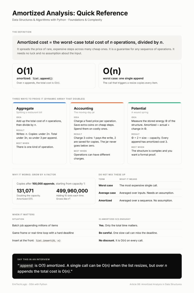
The amortized cost of an operation is the worst-case total cost of any sequence of n operations, divided by n.
When you hear “amortized O(1)” (also written “O(1) amortized”), it means this: any sequence of n operations costs O(n) in total. Each operation is O(1) on average over that sequence, even if one of them is slow.
Three points make this idea easy to remember:
- It is a guarantee, not a guess. The bound holds for the worst possible sequence of operations. There is no luck and no probability in it.
- It describes a sequence, not one call. A single call can still be slow. The promise is about the group.
- Expensive steps must be rare. Each costly step has to be “paid for” by many cheap steps that came before it.
In the last article, you analyzed one function call at a time. You counted loops, nested loops, and recursion for a single run. Amortized analysis steps back. It asks what happens when you call the same operation again and again on the same data structure.
Why Average Cost Isn’t the Same as Average Case
The word “average” causes the most confusion here. Amortized cost and average-case cost both sound like “the usual cost.” They are not the same thing.
A coffee shop shows the difference well.
- Average case: On a normal day, a coffee takes about 2 minutes. That number depends on the customers. If a huge group walks in with complicated orders, the average falls apart.
- Amortized: Once a day, the machine needs a 20-minute cleaning. That is fixed. Even on the worst possible day, 100 coffees take at most 100 × 2 + 20 = 220 minutes. That is about 2.2 minutes per coffee. You did not need to guess anything about the customers.
The first one is a bet on typical inputs. The second one is a promise that holds for every sequence.
| Average-case analysis | Amortized analysis | |
|---|---|---|
| What gets averaged? | Many different possible inputs | Many operations in a row on one data structure |
| Does it use probability? | Yes. It assumes how inputs are spread out | No |
| Can unlucky input break it? | Yes | No |
| What does it promise? | The expected cost | The worst-case total cost, divided by the number of operations |
| Python example | Looking up a key in a dict | list.append() |
A dictionary lookup is O(1) on average because it assumes a good spread of hash values. If many keys collide, lookups slow down. That is an average-case claim.
A list append is O(1) amortized because of how the list grows. It does not depend on what values you append, or in what order. That is an amortized claim.
Rule to remember: average-case needs an assumption about the input. Amortized analysis needs no assumption about the input. It only needs a sequence of operations on the same structure.
Dynamic Array Example: The Bookshelf That Keeps Growing
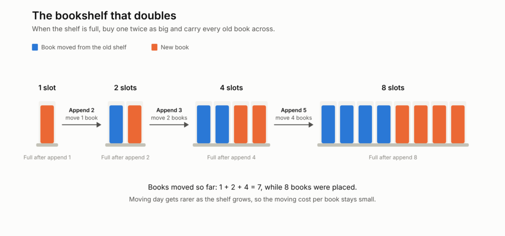
Picture a bookshelf with one slot. You place your first book there. The shelf is now full.
When you buy the second book, there is no room. So you do this:
- Buy a new shelf that is twice as big.
- Carry every old book to the new shelf.
- Place the new book.
- Throw away the old shelf.
Moving day is painful. But look at what you get. The new shelf has empty slots, so the next few books are easy. You just place them. When the shelf fills up again, you buy one twice as big again.
This is how a dynamic array works. A plain array needs one continuous block of memory, so it cannot simply stretch. A dynamic array hides this. It keeps some free slots at the end. When they run out, it allocates a bigger block and copies everything over. Python’s list is a dynamic array.
The Python code
Here is a small dynamic array. It doubles its capacity when it is full. It also counts how many items it copies, so we can measure the cost.
class DynamicArray:
    def __init__(self):
        self.capacity = 1
        self.size = 0
        self.data = [None] * self.capacity
        self.copies = 0  # how many items we have moved so far

    def append(self, value):
        if self.size == self.capacity:
            self._resize(self.capacity * 2)
        self.data[self.size] = value
        self.size += 1

    def _resize(self, new_capacity):
        new_data = [None] * new_capacity
        for i in range(self.size):
            new_data[i] = self.data[i]
            self.copies += 1
        self.data = new_data
self.capacity = new_capacityThe logic is short:
- If there is room,
appendwrites the value and finishes. That is one step. - If the array is full,
_resizeruns first. It copies every item, one by one.
Watch the cost of each append
Let’s call the cost of an append “1 for the write, plus 1 for every item copied.” Here is what happens as we append items one by one.
| Append # | Size after | Capacity after | Items copied | Cost |
|---|---|---|---|---|
| 1 | 1 | 1 | 0 | 1 |
| 2 | 2 | 2 | 1 | 2 |
| 3 | 3 | 4 | 2 | 3 |
| 4 | 4 | 4 | 0 | 1 |
| 5 | 5 | 8 | 4 | 5 |
| 6 | 6 | 8 | 0 | 1 |
| 7 | 7 | 8 | 0 | 1 |
| 8 | 8 | 8 | 0 | 1 |
| 9 | 9 | 16 | 8 | 9 |
| … | … | … | … | … |
| 17 | 17 | 32 | 16 | 17 |
Look at the pattern in the Cost column. The expensive appends are number 2, 3, 5, 9, and 17. They happen right after the size hits 1, 2, 4, 8, and 16. The gaps between them keep doubling. So the costly steps get rarer as the array grows, and each one is paid for by a longer run of cheap appends.
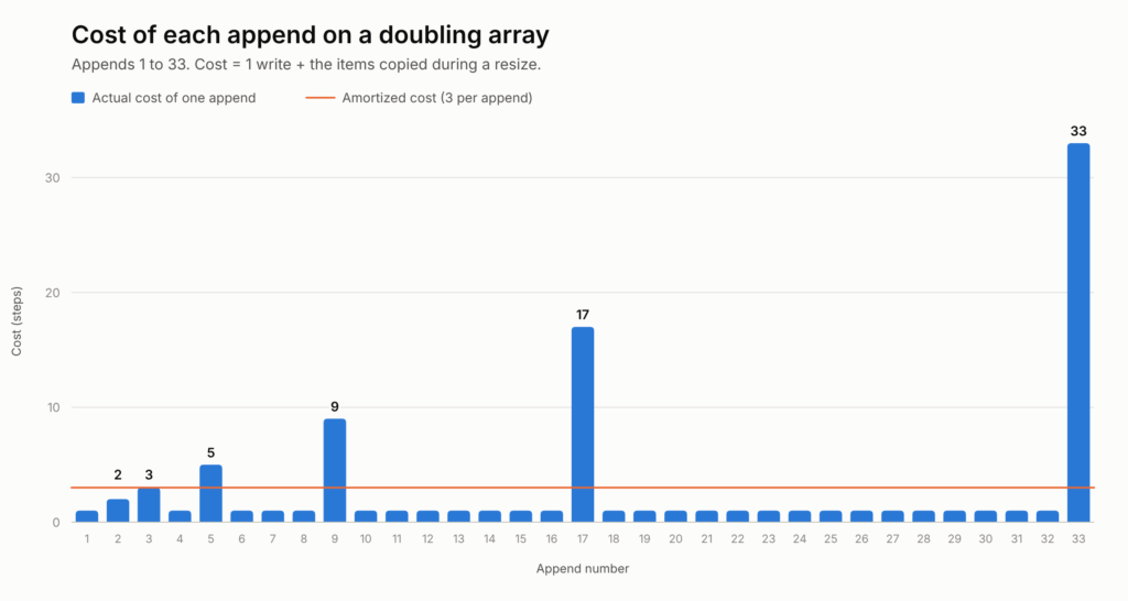
Now let’s measure the cost per append for bigger inputs.
for n in (10, 100, 1_000, 100_000):
    arr = DynamicArray()
    for i in range(n):
        arr.append(i)
    total_cost = n + arr.copies  # n writes + all the copies
print(f"n={n:>7,} total cost={total_cost:>9,} per append={total_cost / n:.2f}")Output:
n=     10  total cost=       25  per append=2.50
n=    100  total cost=      227  per append=2.27
n=  1,000  total cost=    2,023  per append=2.02
n=100,000  total cost=  231,071  per append=2.31
The input grew 10,000 times bigger, from 10 to 100,000. The cost per append stayed between 2 and 3. It did not grow. That flat line is what “amortized O(1)” looks like in practice.
| Operation | Worst case (one call) | Amortized |
|---|---|---|
append | O(n) | O(1) |
| Read by index | O(1) | O(1) |
| Extra space | O(n) | O(n) |
The worst case for one append is O(n), because a resize copies n items. Over a long run, though, each append costs O(1) on average. The next three sections explain why that is always true, using three different methods.
Python List Append: What Really Happens
Your DynamicArray doubles its size. Does Python’s real list do the same? Not exactly, but it follows the same idea.
A Python list keeps its items in one continuous block of memory. Each slot holds a reference to an object, so copying a slot copies a reference, not the object itself. When append finds no free slot, CPython asks for a bigger block. It also asks for extra room on purpose. This is called over-allocation.
You can see it with sys.getsizeof():
import sys

items = []
last_size = sys.getsizeof(items)
print(f"len=0 -> {last_size} bytes")

for i in range(1, 65):
    items.append(i)
    size = sys.getsizeof(items)
    if size != last_size:  # the list just got a bigger block
        print(f"len={i:>2} -> {size} bytes")
last_size = sizeHere is the output from CPython 3.13 on a 64-bit machine:
len=0 -> 56 bytes
len= 1 -> 88 bytes
len= 5 -> 120 bytes
len= 9 -> 184 bytes
len=17 -> 248 bytes
len=25 -> 312 bytes
len=33 -> 376 bytes
len=41 -> 472 bytes
len=53 -> 568 bytes
The size does not change on every append. It jumps only at len = 1, 5, 9, 17, 25, 33, 41, and 53. Between those jumps, appends use free slots that were already reserved. Each slot takes 8 bytes. So the list has room for 4, 8, 16, 24, 32, 40, 52, and 64 items at each step.
The growth is about 12.5% plus a few extra slots. It is not an exact doubling. The exact numbers are an implementation detail. They can differ between Python versions and between implementations such as PyPy. What matters is the shape: each new block is a constant factor bigger than the old one.
Why growing by a factor matters
What if the list grew by a fixed amount instead, say 10 slots each time? Let’s count the copies.
def count_copies(n, grow):
    capacity, size, copies = 1, 0, 0
    for _ in range(n):
        if size == capacity:
            copies += size           # copy every item
            capacity = grow(capacity)
        size += 1
    return copies

for n in (1_000, 10_000, 100_000):
    doubling = count_copies(n, lambda c: c * 2)
    add_ten = count_copies(n, lambda c: c + 10)
print(f"n={n:>7,} doubling={doubling:>9,} add 10={add_ten:>12,}")Output:
n=  1,000  doubling=    1,023  add 10=      49,600
n= 10,000  doubling=   16,383  add 10=   4,996,000
n=100,000  doubling=  131,071  add 10= 499,960,000
Look at the last row. Doubling copies about 131 thousand items. Adding 10 slots copies about 500 million. Adding a fixed amount means a resize every 10 appends, and each resize copies everything so far. The total grows like n², so the cost per append grows with n. It is not amortized O(1).
Key idea: amortized O(1) appends need geometric growth. The list must grow by a factor, not by a fixed number of slots.
This is also why the Python wiki lists list.append() as O(1) in the Python time complexity table, under the “amortized worst case” heading.
Aggregate Analysis: Add Everything Up, Then Divide
We saw that the cost per append stays flat. Now let’s prove it. There are three standard ways to do that. Aggregate analysis is the simplest, so we start here.
The idea is the same as splitting a restaurant bill:
- Find the total cost of n operations, in the worst case.
- Divide the total by n.
That’s it. Every operation gets the same amortized cost.
Aggregate analysis of the dynamic array
Take n appends on a dynamic array that doubles when full.
- Writes: Every append writes one item. That is n writes in total.
- Copies: A resize happens when the size is 1, 2, 4, 8, and so on. Each resize copies that many items.
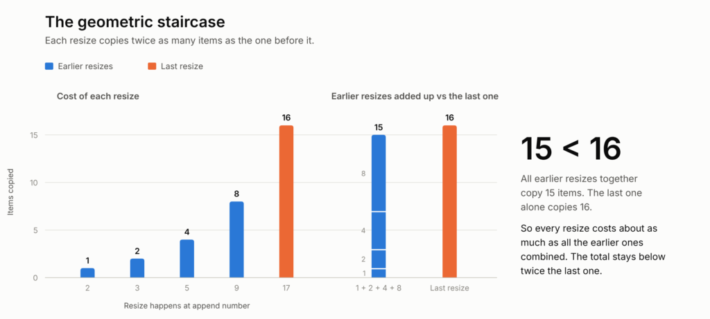
So the total number of copies is:
1 + 2 + 4 + 8 + ... + 2^k where 2^k < nThis sum equals 2^(k+1) − 1, which is less than 2n. Here is a quick check with n = 9. The copies are 1 + 2 + 4 + 8 = 15. The writes are 9. The total is 24, and 3n is 27.
Now put the two parts together:
total cost = writes + copies < n + 2n = 3n
amortized cost per append = total cost / n < 3 = O(1)
Why is the sum so small? Look at the sizes of the resizes. Each one is exactly half of the next one: 1, 2, 4, 8, 16. The last resize copies at most n items, and at least half of n. The one before it copies half as many. The one before that copies a quarter as many. The last step is as big as all the earlier steps put together. So the whole sum stays below twice the last term, and that is below 2n.
You can also check this claim with code. This test uses the DynamicArray from earlier:
arr = DynamicArray()
for n in range(1, 10_001):
    arr.append(n)
    assert n + arr.copies <= 3 * n  # total cost never passes 3n

print("Total cost stayed under 3n for every n up to 10,000")It runs without an error. The total cost never passes 3n.
When to use it: aggregate analysis is perfect when you have one operation, or when every operation can share one average cost. When a structure has several different operations, the next two methods give you more control.
Accounting Method: Pay a Little Extra Now
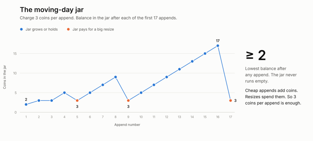
Back to the bookshelf. Imagine you keep a jar labeled “moving day.” Every time you buy a book, you drop a few extra coins into the jar. On moving day, you pay for the move out of the jar. If the jar never runs empty, your plan works.
The accounting method (also called the banker’s method) turns this idea into rules:
- Pick a fixed charge for each operation. This is the amortized cost you claim.
- If the real cost is less than the charge, save the difference as credit in a bank.
- If the real cost is more than the charge, pay the difference from the bank.
- The bank must never go below zero.
If the bank never goes negative, the charge is a valid amortized cost. The total real cost can never be more than the total charges.
Charging 3 coins per append
Let’s charge 3 coins for every append. Here is how each append spends its coins:
- 1 coin pays for writing the item now.
- 1 coin is saved on the new item. It will pay for copying that item at the next resize.
- 1 coin is saved on the new item too. It will pay for copying one old item, one that has already used up its own coin.
Why does this work? Say the array has room for C items and is now full. Half of those items are new since the last resize. Each of them saved 2 coins, so the bank holds C coins. A resize copies C items. The bank pays for it exactly.
Here is the bank for the first 9 appends:
| Append # | Real cost | Charge | Bank after |
|---|---|---|---|
| 1 | 1 | 3 | 2 |
| 2 | 2 | 3 | 3 |
| 3 | 3 | 3 | 3 |
| 4 | 1 | 3 | 5 |
| 5 | 5 | 3 | 3 |
| 6 | 1 | 3 | 5 |
| 7 | 1 | 3 | 7 |
| 8 | 1 | 3 | 9 |
| 9 | 9 | 3 | 3 |
The bank goes up on cheap appends. It drops on expensive ones. It never goes below zero. So 3 is a valid amortized cost, and every append is O(1) amortized.
Test it in Python
def check_accounting(n, charge=3):
    capacity, size, bank = 1, 0, 0
    for _ in range(n):
        cost = 1                 # writing the new item
        if size == capacity:     # array is full: copy every item
            cost += size
            capacity *= 2
        size += 1
        bank += charge - cost    # save extra coins, or spend saved ones
        assert bank >= 0, "ran out of credit"
    return bank

print(check_accounting(1_000))
print(check_accounting(100_000))Output:
977
68929
The function returns the coins left at the end. The assert would stop the program if the bank ever dropped below zero. It never does.
What if we charge only 2 coins?
check_accounting(1_000, charge=2)
# AssertionError: ran out of credit
The jar runs dry at the 5th append. Two coins are not enough. That tells us something useful: the charge cannot be a random guess. It must be big enough to cover the future copies.
Potential Method: Energy Stored in the Data Structure
The third method is a little more abstract. Think of a spring. Every time you push it a bit, it stores energy. Later, one sudden release lets out all that stored energy at once.
A dynamic array behaves in a similar way. Each cheap append “winds the spring” a little. The expensive resize “releases the spring.”
The potential method puts a number on this stored energy. It works like this:
- You define a potential function, written Φ (the Greek letter phi). It looks at the current state of the data structure and returns a number.
- The amortized cost of an operation is:
amortized cost = actual cost + Φ(after) − Φ(before)- Φ must never end lower than where it started.
Why does this work? When you add up the amortized costs of many operations, the Φ terms cancel out in the middle. Only the first and the last Φ remain. So the total amortized cost is at least the total real cost.
Choosing Φ for the dynamic array
The trick is to pick a good Φ. For the dynamic array, this one works:
Φ = 2 × size − capacityHere is the idea behind it. Right after a resize, the array is only about half full, so Φ is small. Each append raises Φ by 2. When the array is full, Φ equals the number of items. That is exactly the number of items the next resize must copy. The stored energy matches the coming bill.
A normal append (there is room):
- Actual cost is 1.
- The size grows by 1, so Φ grows by 2.
- Amortized cost = 1 + 2 = 3.
A resizing append (the array is full with c items):
- Φ before = 2c − c = c.
- Actual cost = c copies + 1 write = c + 1.
- After the resize, the size is c + 1 and the capacity is 2c. So Φ after = 2(c + 1) − 2c = 2.
- Amortized cost = (c + 1) + (2 − c) = 3.
Both cases give 3. The big cost of copying c items is cancelled by the big drop in Φ. So every append is O(1) amortized.
Here are the first 9 appends, step by step:
| Append # | Actual cost | Φ before | Φ after | Amortized cost |
|---|---|---|---|---|
| 1 | 1 | −1 | 1 | 3 |
| 2 | 2 | 1 | 2 | 3 |
| 3 | 3 | 2 | 2 | 3 |
| 4 | 1 | 2 | 4 | 3 |
| 5 | 5 | 4 | 2 | 3 |
| 6 | 1 | 2 | 4 | 3 |
| 7 | 1 | 4 | 6 | 3 |
| 8 | 1 | 6 | 8 | 3 |
| 9 | 9 | 8 | 2 | 3 |
The actual cost jumps between 1 and 9. The amortized cost is a calm 3 every time. (Φ starts at −1 in this code, because the empty array already owns one free slot. That small offset does not matter, since Φ ends higher than it started.)
Test it in Python
def phi(size, capacity):
    return 2 * size - capacity   # the potential function

def check_potential(n):
    capacity, size = 1, 0
    for _ in range(n):
        before = phi(size, capacity)
        cost = 1                 # writing the new item
        if size == capacity:     # full: copy every item
            cost += size
            capacity *= 2
        size += 1
        after = phi(size, capacity)
        amortized = cost + after - before
        assert amortized <= 3, f"amortized cost was {amortized}"
    print(f"Every append had an amortized cost of at most 3 ({n:,} appends)")

check_potential(100_000)Output:
Every append had an amortized cost of at most 3 (100,000 appends)Which method should you use?
All three methods prove the same result for the dynamic array. They differ in how they think about it.
| Method | Main idea | Real-world picture | Best when |
|---|---|---|---|
| Aggregate | Total cost of n operations, divided by n | Splitting a restaurant bill | There is one kind of operation |
| Accounting | Charge extra on cheap steps, keep the credit | The “moving day” jar | Different operations can have different charges |
| Potential | Measure the stored energy of the structure | A wound spring | The structure is complex and you want a formal proof |
In interviews, aggregate analysis and the accounting method are the easiest to explain out loud. Reach for the potential method when the first two feel awkward.
A Second Example: A Queue Built From Two Stacks
Amortized analysis is not only about lists. It shows up whenever a costly step is rare and each item pays for it only once. A classic interview problem shows this well: build a queue using two stacks.
Here is a picture from an office. You have two trays of paper.
- New papers go on top of the inbox tray. The newest paper is always on top.
- When you need the oldest paper, it is stuck at the bottom of the inbox.
- So you flip the whole inbox onto the outbox tray. The order reverses, and now the oldest paper is on top.
- You take papers from the outbox until it is empty. Only then do you flip the inbox again.
Flipping the tray takes a while. But each paper gets flipped only once.
class TwoStackQueue:
    def __init__(self):
        self.inbox = []
        self.outbox = []

    def enqueue(self, item):
        self.inbox.append(item)

    def dequeue(self):
        if not self.outbox:               # outbox is empty: flip the inbox
            while self.inbox:
                self.outbox.append(self.inbox.pop())
        if not self.outbox:
            raise IndexError("dequeue from empty queue")
        return self.outbox.pop()

q = TwoStackQueue()
for i in range(1, 6):
    q.enqueue(i)

print([q.dequeue() for _ in range(3)])   # [1, 2, 3]
q.enqueue(6)
print([q.dequeue() for _ in range(3)]) # [4, 5, 6]The items come out in first-in, first-out order, just like a real queue.
The cost of dequeue
One dequeue can be slow. If the outbox is empty and the inbox holds n items, that single call moves all n of them. So the worst case for one call is O(n).
Now count the work per item instead. Every item goes through exactly four steps in its life:
- It is pushed onto the inbox.
- It is popped off the inbox.
- It is pushed onto the outbox.
- It is popped off the outbox.
That is at most 4 basic steps per item, no matter what order the calls come in. So m operations cost at most about 4m steps in total. That is aggregate analysis again. Each enqueue and dequeue is O(1) amortized.
The accounting view gives the same answer. Charge 3 coins for each enqueue. One coin pays for the push now. The other two stay with the item to pay for its later move from the inbox to the outbox. A dequeue is charged 1 coin for the final pop.
This queue is a teaching tool. In real Python code, use collections.deque, which is built for this job. You will meet it in the stacks and queues cluster of this series.
Amortized vs Worst-Case Complexity
Think about your daily drive to work. It takes 20 minutes on a normal day. Once a month, a road closure adds 2 hours.
- The worst case for one trip is 2 hours 20 minutes.
- The amortized cost over a month is close to 24 minutes per trip. You add up all the trips and divide.
Both numbers are true. They answer different questions. The first one is about your worst single day. The second is about your month as a whole.
| Worst-case complexity | Amortized complexity | |
|---|---|---|
| What it measures | The most expensive single call | The total cost of many calls, divided by the number of calls |
| Guarantee | Holds for every single call | Holds for the whole sequence, not each call |
| Can one call be slow? | No. That is the bound | Yes, but slow calls are rare |
Example: list.append() | O(n), when a resize happens | O(1) |
An important rule: amortized cost is never larger than worst-case cost. It can be much smaller, as it is for append.
Here is how a few operations look in both views:
| Operation | One call, worst case | Amortized |
|---|---|---|
list.append(x) | O(n) | O(1) |
list[i] (read by index) | O(1) | O(1) |
list.insert(0, x) | O(n) | O(n) |
TwoStackQueue.dequeue() | O(n) | O(1) |
Notice insert(0, x). It shifts every item one place to the right, on every call. There is no rare expensive step and no cheap majority. So amortized analysis gives no discount here.
In an interview, say both numbers together:
“
appendis O(1) amortized. A single call can be O(n) when the list resizes, but over n appends the total cost is O(n).”
That one sentence shows you know the difference.
When Amortized Analysis Matters
Amortized analysis is not just a classroom exercise. You will meet it in three places.
1. When you study built-in data structures. A Python list resizes as it grows. Hash tables, which sit behind dict and set, also resize as they fill up. Their costs are described with amortization too. Later in this series, Union-Find (the disjoint set structure) is another example. Its famous speed comes from an amortized argument.
2. When you answer interview questions. Interviewers like to ask, “What is the complexity of append?” A good answer names both the single-call cost and the amortized cost.
3. When you analyze an algorithm that looks slower than it is. Some algorithms have a loop inside a loop, yet they run in O(n). The inner work is shared across the whole run. You will see this clearly in the next section.
When amortized O(1) is not enough
Remember the commute? If you have a flight to catch on the day of the road closure, the 24-minute average does not help you. The 2 hours 20 minutes matters.
Code has the same problem. An amortized bound says nothing about one unlucky call. That call pays the full price of the resize. In most programs, this is fine. In some programs, it is not.
| Situation | Is amortized O(1) enough? | Why |
|---|---|---|
| A batch job that appends millions of items | Yes | Only the total running time matters |
| A web handler that appends a few items to a list | Yes | The list is small, so a resize is cheap |
| A game loop with a fixed time budget per frame | Be careful | One slow call can make a frame late |
| Real-time audio or a control loop with hard deadlines | No | Every single call must meet the deadline |
If you know the final size in advance, you can skip the problem. Reserve the space first, then fill it:
# Reserve space once. No resize can happen while we fill it.
buffer = [None] * 1_000_000
for i in range(1_000_000):
buffer[i] = iThe rule of thumb is simple. If total time matters, amortized analysis is the right tool. If the delay of a single call matters, look at the worst case.
How to Recognize Amortized Patterns in a DSA Problem
In the last article, you learned a rule: nested loops multiply. That rule is correct most of the time. However, there is one famous exception. Sometimes a loop sits inside another loop, and the total work is still O(n). Here is how to spot those cases.
| Clue in the problem or code | What it usually means |
|---|---|
A while loop inside a for loop, but the inner index never moves backward | Two pointers or a sliding window |
A while loop that pops from a stack inside a for loop | A monotonic stack |
| A structure that resizes, rehashes, or rebuilds itself now and then | Amortized cost per operation |
| Each item enters a structure once and leaves it once | Count entries and exits to get the total |
A worked example: days until a warmer day
You have a list of daily temperatures. For each day, you want to know how many days you must wait for a warmer day. If there is none, the answer is 0.
def days_until_warmer(temps):
    answer = [0] * len(temps)
    stack = []  # indexes of days still waiting for a warmer day
    for i, t in enumerate(temps):
        while stack and temps[stack[-1]] < t:
            j = stack.pop()
            answer[j] = i - j
        stack.append(i)
    return answer

print(days_until_warmer([30, 31, 29, 28, 33])) # [1, 3, 2, 1, 0]The code has a while loop inside a for loop. By the nested-loop rule, it looks like O(n²). It is not.
Here is the trick. Do not count the work per loop. Count how many times each item can be touched in total:
- Every day is pushed onto the stack exactly once.
- Every day is popped off the stack at most once.
So the while loop can run at most n times in total, across the whole for loop. Not n times per day. The total work is O(n) for the whole list. That is O(1) amortized per day.
Think of a ticket counter. Each customer joins the line once and leaves it once. It does not matter how the line moves during the day. The total number of joins and leaves is fixed.
Key idea: when a nested loop looks too slow, ask one question. “How many times can each item be pushed, popped, or visited in total?” If the answer is a small constant, the whole algorithm is linear.
You will use this idea again in these guides: Two Pointers, Sliding Window, and Monotonic Stack. Each of them gets its own full article in this series.
Common Mistakes with Amortized Analysis
These are the slips that cost people points in interviews and cause bugs in real code.
| Mistake | Why it is wrong | How to avoid it |
|---|---|---|
| Saying “append is always O(1)” | One append can copy the whole list | Say “O(1) amortized, O(n) worst case for a single call” |
| Mixing up amortized and average case | Average case needs an assumption about the input. Amortized does not | Ask: “Does this claim depend on lucky input?” If yes, it is average case |
| Growing by a fixed amount | The total copying becomes O(n²), as the “add 10” test showed | Grow by a factor, such as 1.5× or 2× |
| Treating every list operation as amortized O(1) | insert(0, x) and pop(0) shift every item on every call | Use collections.deque for work at the front |
| Calling every nested loop O(n²) | A loop with shared work, like a monotonic stack, is O(n) | Count how many times each item can be touched in total |
| Moving items back and forth in the two-stack queue | Flipping on every call destroys the bound | Flip only when the outbox is empty |
The front-of-the-list trap
This one deserves a closer look, because it is easy to write by accident.
from collections import deque

line = deque([1, 2, 3])
line.popleft()        # O(1): removes from the front without shifting

items = [1, 2, 3]
items.pop(0) # O(n): every remaining item shifts one place leftBoth lines remove the first item. The list version looks harmless. In a loop over a large list, it quietly turns an O(n) job into an O(n²) job.
Edge cases to remember
- The first append. An empty list has no free slots, so the first append always allocates.
- Shrinking. If a structure shrank the moment it dropped below full, a push, pop, push, pop pattern at the boundary would resize on every call. Real implementations avoid this. CPython shrinks a list only when it falls below half of its allocated space.
- Copy-heavy operations. Slicing,
list(items), anditems + othercopy the data. Each is O(n) on every call, with no amortized discount.
FAANG-Style DSA Interview Questions on Amortized Analysis
These eight questions come up again and again. Practice saying the answers out loud.
1. What does “amortized O(1)” mean?
It means that any sequence of n operations costs O(n) in total. So the average cost per operation is constant, even if a few single operations are expensive. It is a guarantee for the worst possible sequence, not a bet on lucky input.
2. Why is list.append() O(1) amortized and not O(1) in the worst case?
When the list runs out of free slots, Python allocates a bigger block and copies every item. That single call costs O(n). But the list grows by a factor each time, so these resizes get rarer as the list grows. Over n appends, the total cost stays O(n).
3. How is amortized analysis different from average-case analysis?
Average-case analysis averages over possible inputs, and it needs an assumption about how those inputs are spread. Amortized analysis averages over a sequence of operations on one structure, and it needs no assumption at all. Amortized bounds hold even for the worst possible sequence.
4. Why must a dynamic array grow by a factor instead of a fixed amount?
If it grows by a fixed amount, such as 10 slots, it resizes every 10 appends. Each resize copies everything so far. The total copying grows like n², so appends are no longer O(1) amortized. Growing by a factor, such as 2×, makes the copy sizes form a geometric series that adds up to O(n).
5. What are the three methods of amortized analysis?
Aggregate analysis finds the total cost of n operations and divides by n. The accounting method charges extra on cheap operations and saves the credit to pay for costly ones. The potential method defines a function of the data structure’s state, and adds its change to the actual cost.
6. What is the amortized cost of dequeue in a queue made from two stacks?
O(1) amortized. One call can move all n items from the inbox to the outbox, which is O(n). But each item is pushed and popped at most twice in total, once on each stack. So m operations cost O(m) overall.
7. A for loop contains a while loop that pops from a stack. Is the time O(n²)?
Usually not. Each item is pushed once and popped at most once. So the while loop runs at most n times across the whole for loop, and the total is O(n). Say this out loud, because it shows you count work per item, not per loop.
8. Can an operation be O(1) amortized and still be a bad choice?
Yes. Amortized O(1) says nothing about one slow call. In a real-time system, such as audio processing or a game frame with a fixed time budget, one resize can miss a deadline. In those cases, reserve the space in advance or pick a structure with steady per-call cost.
Frequently Asked Questions
Is inserting into a Python
dictorsetalso amortized O(1)?Mostly, yes. Hash tables grow as they fill up, and the occasional resize rebuilds the table. The Python wiki lists
dictandsetinserts as O(1) on average, with a worst case of O(n). The “average” there also depends on a good spread of hash values, which is an average-case idea, not a purely amortized one.Does
list.pop()have an amortized cost too?Popping from the end is O(1). CPython also shrinks the list’s memory only when the list falls below half of its allocated space. That keeps shrinking rare, so repeated pushes and pops do not cause constant resizing.
Can an amortized cost be something other than O(1)?
Yes. Amortized bounds can take any form. For example, splay trees are known for O(log n) amortized operations. The word “amortized” only tells you that the bound is averaged over a sequence.
Do I need to prove amortized bounds in an interview?
Usually not a full proof. A short reason is enough. For example: “The list doubles in size, so the copies add up to about 2n over n appends, which is O(1) per append.” That is aggregate analysis in one sentence.
Is the potential function always 2 × size − capacity?
No. That Φ belongs to the dynamic array. Each data structure needs its own. A good Φ is small right after an expensive step and large just before the next one. That way, its drop pays for the expensive step.
Does over-allocation waste memory?
A little. This is the same trade-off you saw in the last article: spend extra memory to save time. For large lists, CPython reserves roughly an eighth more room than the list needs, plus a few slots. A simple doubling array can leave up to half of its space empty. Both choices keep appends fast.
Conclusion: From Amortized Analysis to Arrays
Amortized analysis answers a simple question: what does one operation cost over a long run? You add up the total cost of many operations, in the worst case, and divide by the number of operations. That is why list.append() is O(1) amortized, even though one call can copy the whole list.
You also have three tools for proving it. Aggregate analysis adds everything up and divides. The accounting method saves coins on cheap steps to pay for costly ones. The potential method tracks the energy stored in the structure. All three agree that a doubling array costs about 3 per append.
From now on, say both numbers when you describe an operation. For example: “append is O(1) amortized and O(n) in the worst case for a single call.” That one sentence shows you understand how the structure really works.
What Cluster 1 gave you
This article closes the Foundations & Complexity cluster. Here is how the five articles fit together:
| Article | The skill you gained |
|---|---|
| What Is Big O Notation? | A language for how cost grows with input size |
| Best, Average, and Worst-Case Time Complexity | Knowing which case you are talking about |
| Recursion in Python | Reading the call stack and the recursion tree |
| How to Analyze the Time and Space Complexity of an Algorithm | A repeatable process for any piece of code |
| Amortized Analysis (this article) | Judging operations that are cheap most of the time |
You now have the full toolkit for measuring code. Therefore, it is time to apply it to real data structures.
What to read next
The next cluster is Arrays & Strings. It starts with Arrays in Python: Operations, Complexity, and Common Patterns. You already know why append is cheap and why insert(0, x) is not. The next article builds on that and shows how arrays behave in everyday code.
If you want to see the whole path at once, the DSA with Python guide lays out every stage of the roadmap, from complexity to interview preparation.
Official External Resources
- Python Wiki: Time Complexity: the reference table of costs for Python’s built-in data structures, including the “amortized worst case” column.
- CPython source: listobject.c: the real implementation of the list type, including how it over-allocates when it resizes.
- Python Documentation: collections.deque: the official description of the double-ended queue, the right tool for work at the front of a sequence.
- MIT OpenCourseWare: Amortization and Amortized Analysis: a lecture from MIT’s algorithms course on the methods covered in this article.






Leave a Reply